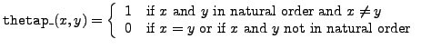
André Heck
Draft: Amsterdam, October 2000
©2000, A.J.P. Heck and J.A.M. Vermaseren
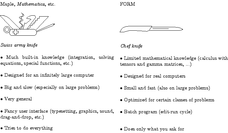
The origin of computer algebra is high energy physics, where the need for algebra engines to handle big computations was felt earliest. The programs REDUCE and SCHOONSCHIP were born in the sixties. REDUCE transformed gradually into a general purpose system and can be considered as one of the predecessors of the modern general purpose systems such as Maple and Mathematica. The design of such general purpose systems make them useful for various areas, but when it comes to really large computations they are too slow, use too big memory, and so on. SCHOONSCHIP was a program completely dedicated towards and optimized for large computations in high energy physics: it was written in assembler language and operated fast. SCHOONSCHIP can be considered as the predecessor of the FORM program.
FORM has been designed along the same philosophy: make a symbolic manipulation program that is useful for ``real computations'' on ``real computers''. FORM has been developed over the last fifteen years by Jos Vermaseren at NIKHEF. The first version was released in 1989 and made available by anonymous ftp from ftp.nikhef.nl. The second enhanced version, FORM 2, was commercially released in 1991. The present release FORM 3 is the next major improvement of the software. FORM3 is not only useful for computations in high energy physics (the original application area), but it is also well-suited for large symbolic manipulations of general nature, in cases where other systems give up. Pattern matching in formula manipulation and computing in noncommutative algebras are two other examples of application areas outside the field of high energy physics where FORM has proved to be champion in symbol crunching.
Before starting to learn FORM, let us compare the program with other general purpose systems such as Maple and Mathematica so that it is clear where and why FORM is different. The following comparison originates from a short course on FORM [Oldenborgh 95].
In order to do a calculation in FORM, you have to write a program, store it in a file, and call FORM with this file as an argument. Let us look at a simple example.
Suppose you have a file sample1.frm with the following contents.
    Symbols a,b;
    Local [(a+b)^2] = (a+b)^2;
    Print;
    .end
When you call FORM by form sample1, the following will
appear on your terminal screen.
    FORM version 3.-(Nov 29 1997). Run at: Tue Jan  6 19:15:59 1998
    Symbols a,b;
    Local [(a+b)^2] = (a+b)^2;
    Print;
    .end

Time =       0.10 sec    Generated terms =          3
        [(a+b)^2]        Terms in output =          3
                         Bytes used      =         52

   [(a+b)^2] =
      2*a*b + a^2 + b^2;
Let us have a closer look at the above session.
The basic object in FORM is a term.
Formulae consist of terms, and terms are separated by addition
and subtraction. If a formula contains parentheses
these are immediately removed as in our example: the formula [(a+b)^2]
contains three terms. Note that objects have to be declared
in FORM before they can be used. The first line informs the system that
a and b are algebraic symbols. The second line defines
[(a+b)^2] as a local expression that has to be manipulated. The
Print statement is necessary to see the result. The
word .end marks the end of the program: it is for
FORM the signal to execute the last program block and to finish afterwards.
FORM shows the original program and the runtime statistics on the screen.
Some general remarks about a regular FORM program:
frm.
Symbols, Local, Print, and .end, and
some continuation. FORM statements can be continued over
several lines, but they must end with a semicolon.
You can also have more than one statement in a program line.
Symbols and Symbol are equally
valid, and for FORM Indices and Index are the same.
Symbols you can just use S, and Local can
be abbreviated as L. For clarity of the examples, we have not
used the abbreviation possibilities of FORM in this tutorial.
alpha,
a1, H2O, and firstExercise are valid names. If you want
to use spaces in a name for reasons of readability, or if you want to use
special characters such as dots, colons, or slashes, then you must surround
the name with square brackets
-l in
the starting command: if in our example we had said form -l sample1, the
effect would have been the creation of the file sample1.log with the
contents that normally appears on the screen.
Local [(a+b)^2] = (a+b)^2 statement in the first example by
Local [(a+b)^2] = (a+b)*(a+b) ?
Symbols a,b
declaration in the first example by
Functions a,b ?
    Symbol a;
    Functions B, C;
    Local F1 = (a+B+C)^2;
    Local F2 = (a+(B+C))^2;
    Print;
    .end;
What is the difference in working out expression F1 and expression
F2?
    s,t,u; L,F=
    (t+u)
    ^2;
    Print;
    .end
In the second exercise of the last section you have seen
that FORM has an easy way to deal with noncommuting objects,
viz., through the variable type Function.
There are more types in FORM: commuting functions, vectors, and tensors,
to name a few. In this section we shall discuss some of them.
FORM distinguishes between noncommuting
functions, declared by
the keyword Functions, and commuting
functions, declared
by the keyword CFunctions or
Commuting.
The next example clearly demonstrates the difference.
    *
    * Declarations
    *
    Functions f,g;
    CFunctions F,G;
    Symbol x;
    *
    * Specifications, e.g. no runtime statistics
    *
    Off statistics;
    *
    * Definitions
    *
    * local expression with only noncommuting functions
    *
    Local F1 = f(x)*g(x) + g(x)*f(x);
    *
    * Output
    *
    Print;
    *
    * end of module
    *
    .sort

   F1 =
      f(x)*g(x) + g(x)*f(x);

    *
    * local expression with only commuting functions
    *
    Local F2 = F(x)*G(x) + G(x)*F(x);
    Print F2;
    *
    * terminate the program
    *
    .end

   F2 =
      2*F(x)*G(x);
We deliberately made the above example more complicated
than necessary in order to explain some more FORM features.
Off statistics.
Henceforth, it is assumed in all FORM examples that the initialization fileform.setcontains the linenwritestatistics on. This will automatically turn off the printing of runtime messages unless the statementOn statisticsis present in a FORM program.
Symbol,
Function,
statistics,
skip, drop, hide,
Local or Global.
id,
trace, contract,
Print and Bracket.
.sort statement is a directive
to FORM to execute a program block, sort the result (i.e., bring them
in standard ordering), and prepare for further processing.
This brings us to the very short description of how FORM operates; we will come back to this issue in section 1.3. FORM consists of a preprocessor and a compiler. The preprocessor reads from the input stream and prepares input for the compiler. The preprocessor prepares program blocks, also called modules, which are translated by the compiler, and immediately executed. A command for the preprocessor is called a preprocessor instruction. It always starts with the sharp symbol (#), it does not have to end with a semicolon, and it is executed when it is encountered in the input stream. A module is terminated by a statement that starts with a period. Such a statement is called a module instruction. It marks the end of a module, it halts the compiler, and it initiates the execution of the module. Like a preprocessor instruction, a module instructions does not have to end with a semicolon, although it does no harm. The module instructions and their meanings are listed below.
| Instruction | Meaning |
| execute, sort, print, + | |
.sort |
continue |
.end |
terminate |
.clear |
restart softly |
.store |
store globals, remove locals, continue |
There is one other module instruction,
viz., .global.
It makes the definitions and declarations in the module global so that they
cannot be so easily removed again. Most of these directives will be discussed
in later chapters.
Finally, in our example we have used an option of
Print, viz., to print only one expression
instead of all expressions known in the module.
Besides distinguishing commutating and noncommuting functions, FORM can also deal with the following four symmetry properties of functions.
| Symmetry Property | Meaning |
symmetric |
|
antisymmetric |
|
| where
|
|
cyclic |
|
| in the group generated by the cycle
|
|
rcyclic |
|
| in the group generated by the cycle
|
|
| the cycle
|
An example:
    Symbols x1,x2,x3,x4,x5;
    Functions S(symmetric), A(antisymmetric), C(cyclic), R(rcyclic);
    Local [S(x2,x3,x4,x1,x5)] = S(x2,x3,x4,x1,x5);
    Local [A(x2,x3,x4,x1,x5)] = A(x2,x3,x4,x1,x5);
    Local [C(x2,x3,x4,x1,x5)] = C(x2,x3,x4,x1,x5);
    Local [R(x2,x3,x4,x1,x5)] = R(x2,x3,x4,x1,x5);
    Print;
    .end

   [S(x2,x3,x4,x1,x5)] =
      S(x1,x2,x3,x4,x5);

   [A(x2,x3,x4,x1,x5)] =
       - A(x1,x2,x3,x4,x5);

   [C(x2,x3,x4,x1,x5)] =
      C(x1,x5,x2,x3,x4);

   [R(x2,x3,x4,x1,x5)] =
      R(x1,x4,x3,x2,x5);
You see that FORM automatically uses the symmetry properties of the
functions to bring the arguments into standard order (determined
by the order in which objects have been declared). Three remarks:
S(symmetric) into
S(S).
Consider the following FORM session.
    Symbols x,y;
    Commuting f;
    Local F = f(x)+f(x,y)+f(x,,y);
    Print;
    .end

   F =
      f(x) + f(x,y) + f(x,0,y);
Notice that calls of the commuting function f have different number
of arguments. This is a general feature: there is no check on the type
of a function and on the number of arguments in a function call until
something has to be done with the function.
The empty argument in the third call of f is replaced by zero.
In FORM, empty arguments and arguments that are zero are the same.
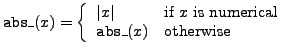
We list the mathematical functions that FORM knows. Like any other built-in object you recognize such a function by its name: it always ends with an underscore. We distinguish between functions that have really been implemented and those whose names have been reserved only. For the latter functions, some safe fixed values and relations may be implemented in future versions of FORM, but do not expect too much of it. Because of potential problems with multivalued functions and with analytic continuations of functions, the number of relations will be limited.
| Implemented Function | Meaning |
abs_ |
absolute value |
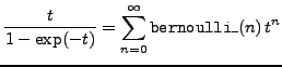
bernoulli_ |
Bernoulli number |
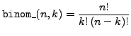
binom_ |
binomial coefficient |
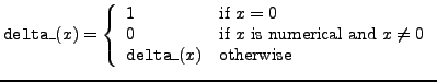
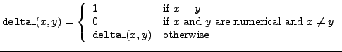
delta_ |
delta function |
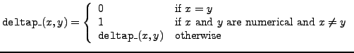
deltap_ |
delta prime function |
fac_ |
factorial |
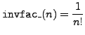
invfac_ |
inverse factorial |
max_, min_ |
maximum and minimum value |
mod_ |
modulo arithmetic of integers |
root_ |
root function |
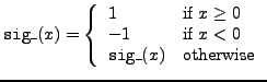
sig_ |
sign function |
sign_ |
signature for integers |
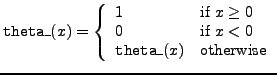
theta_ |
theta function |
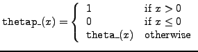
thetap_ |
theta prime function |
| Reserved Function | Meaning |
acos_, asin_, atan_, atan2_ |
inverse trigonometric functions |
acosh_, asinh_, atanh_ |
inverse hyperbolic functions |
cos_, sin_, tan_ |
trigonometric functions |
cosh_, sinh_, tanh_ |
hyperbolic functions |
li2_ |
dilogarithm |
lin_ |
polylogarithm |
ln_ |
natural logarithm |
sqrt_ |
square root function |
Precise definitions of implemented functions are:
 .
.
 .
.
and
So, basically,
![]()

and
So, basically,
![]() and
and
![]()
 .
.
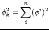
If all ![]() 's in
's in
![]() are
numerical, it evaluates to the minimum value of them. If not, the formula
is returned.
are
numerical, it evaluates to the minimum value of them. If not, the formula
is returned.
and
and
So, basically,
![]() and
and
![]()
The following FORM session illustrates how some of the built-in functions work.
    Symbol x;
    Local F1 = invfac_(3) + x*fac_(3);
    Local F2 = cos_(0) + cos_(x)^2 + sin_(x)^2;
    Local F3 = x^3*sign_(3) + x*abs_(-1/2) + sig_(-3) + sig_(x);
    Local F4 = binom_(5,2) + sqrt_(4) + x*root_(2,4);
    Local F5 = bernoulli_(0) + bernoulli_(1)*x + bernoulli_(2)*x^2;
    Local F6 = max_(1/2,2) + min_(1,x);
    Local F7 = mod_(7,2);
    Print;
    .end;

   F1 =
      1/6 + 6*x;

   F2 =
      sin_(x)^2 + cos_(x)^2 + cos_(0);

   F3 =
       - 1 + 1/2*x - x^3 + sig_(x);

   F4 =
      10 + 2*x + sqrt_(4);

   F5 =
      1 + 1/2*x + 1/12*x^2;

   F6 =
      2 + min_(1,x);

   F7 =
      1;
Vectors are one of the favorite data types of FORM. They can
appear in two ways: with symbolic indices, like in
v(i), and with specific integer indices such as v(1)
and v(2).
In the former case, the indices must be declared. The default dimension of
the underlying vector space is four, but it can be changed by
the Dimension statement.
An example of the use of vectors and indices:
    Vectors u,v;
    Indices i,j;
    Function f;
    Local w1 = u(1) + v(i);
    Local w2 = u(i) * v(j);
    Local w3 = u(i) * u(i);
    Local w4 = v(i) * u(i);
    Local w5 = f(i,j) * u(i) * v(j);
    Print;
    .end

   w1 =
      u(1) + v(i);

   w2 =
      u(i)*v(j);

   w3 =
      u.u;

   w4 =
      u.v;

   w5 =
      f(u,v);
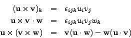
The formulas w3 and w4 show that FORM uses the
so-called Einstein summation convention:
indices that occur twice inside the same
term are considered to be summed over.
So, v(i)*u(i) becomes the inner product or
dot product of u and v, which is
Formula w5 illustrates another convention, called the
SCHOONSCHIP notation, that FORM uses:
when an index is summed over and in one of its occurrences it is the argument
of a vector, then this vector is put at the place of the other
occurrence. In this notation,
![]() ,
where
,
where ![]() is a vector and
is a vector and ![]() some function, is abbreviated as
some function, is abbreviated as ![]() .
.
The automatic summation of indices is also called contraction
of indices.
You can overrule the contraction of indices in
FORM by specifying a zeroth dimension for the index in the declaration.
In this case, explicit summation is still possible by the sum
statement. This statement is also applicable if indices are
arguments of functions or tensors.
    Vector u;
    Index i=0;
    * no contraction over index i
    Local P = u(i) * u(i);
    Print;
    .sort

   P =
      u(i)*u(i);

    sum i;
    Print;
    .sort

   P =
      u.u;

    Function f;
    Local F = f(i);
    sum i,1,3,5;
    Print F;
    .end

   F =
      f(1) + f(3) + f(5);
Keep in mind that FORM does not distinguish between upper (contravariant) and
lower (covariant) indices.
We shall see in the next chapter how this concept from tensor calculus
can be implemented in FORM.
The keyword to declare a tensor in FORM is Tensor or
CTensor. The latter declaration makes clear that FORM assumes
(components of) tensors to be commuting. To declare a noncommuting version
you must use NTensor. Tensors are in FORM special kinds of
functions: their arguments can only be indices and vectors of which it
is assumed that they have been contracted with an index. The advantage is
that the system can manipulate them more efficiently than the general
functions.
In the example below, we consider a sum of two products of tensors and explicitly tell FORM that common indices are summed over. In this way, the system will recognize the equal terms in the expression.
    Tensors S,T;
    Indices i,j,k,l;
    Local F = S(i,k)*T(k,j) + S(i,l)*T(l,j);
    Print;
    .sort

   F =
      S(i,k)*T(k,j) + S(i,l)*T(l,j);

    sum k,l;
    Print;

   F =
      2*S(i,N1_?)*T(N1_?,j);
The dummy index generated by FORM is denoted by a name that ends
with an underscore and a question mark.
FORM has convenience methods to replace tensors by a product of vector
components and vice versa. They are called ToVector
and ToTensor, respectively.
The commands have two arguments, a tensor and a vector.
The order in which these arguments occur is irrelevant.
Replacements from vector to tensor occur not only when
components of the vector are used, but also when the vector is contracted
with other vectors or tensors.
An example that shows it all.
    Tensor t;
    Vector u,v;
    Indices i,j,k;
    Local F1 = v(i)*v(j)*v(k)*v(1);
    Local F2 = v;
    Local F3 = (u.v)^2 * v.v;
    ToTensor v,t;
    Print;
    .sort

   F1 =
      t(1,i,j,k);

   F2 =
      v;

   F3 =
      t(u,u,N1_?,N1_?);

    Local F4 = t;
    ToVector t,v;
    Print;
    .end

   F1 =
      v(1)*v(i)*v(j)*v(k);

   F2 =
      v;

   F3 =
      u.v^2*v.v;

   F4 =
      1;
   FunPowers nofunpowers;
   FunPowers commutingonly;
   FunPowers allfunpowers;
Find out by experimentation what the statements actually do and check also how they affect the printing of powers of tensors.
When writing or studying FORM programs, it is useful to have at least some idea of what FORM internally does. First, you need to know what objects it actually manipulates. The answer is that FORM works with expressions that are sums of terms; each term consisting of a rational coefficient times a product of factors, possibly to some power. The factors can be symbols or more complicated structures such as functions or tensors. The expressions that can be manipulated are called active expressions. There can be many active expressions at the same time.
The method of operation of FORM is as follows.
So, you see that FORM sequentially processes expressions term by term.
This mode of operation means that FORM has no operations that use
more than one term at the same time. For example, a substitution rule like
![]() cannot be expressed as such. You will have to use tricks
such as the replacement rule
cannot be expressed as such. You will have to use tricks
such as the replacement rule
![]() . It also means that there is
no factorization built into FORM because the whole expression must be taken
into account for this mathematical operation. To summarize in one sentence:
. It also means that there is
no factorization built into FORM because the whole expression must be taken
into account for this mathematical operation. To summarize in one sentence:
The examples in this section are to acquaint you with FORM and to show some of its built-in facilities.
FORM provides you of course with tools to compose an expression. For
example, to obtain
![]() you can enter
the following:
you can enter
the following:
    Symbols x,i;
    Local expr = sum_( i, 0, 5, x^i/fac_(i) );
    Print;
    .end

   expr =
      1 + x + 1/2*x^2 + 1/6*x^3 + 1/24*x^4 + 1/120*x^5;
The Levi-Civita tensor or
permutation tensor
![]() plays an important role in tensor calculus.
When the indices range from 1 to
plays an important role in tensor calculus.
When the indices range from 1 to ![]() , it is defined as
, it is defined as
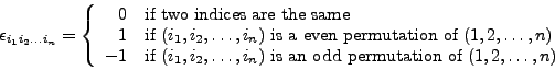
e_.
The product of a pair of Levi-Civita tensors can be rewritten in terms of
Kronecker deltas:
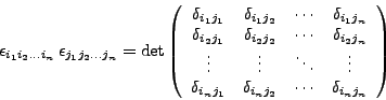
d_(i,j), is defined as
d_ differs from the delta function
delta_. The Kronecker delta has two indices as arguments and serves
as a metric tensor (this implies that it is symmetric).
The second delta function, delta_ has either one or two arguments, which
need not be indices, but can be general expressions. FORM does
not symmetrize the delta function delta_.
The contract statement will do the work of
writing a product of Levi-Civita tensors in terms of Kronecker deltas.
In the example below, the vector space is declared
three-dimensional by the Dimension statement (recall that the default
dimension in FORM is four).
    Dimension 3;
    Indices i,j,k,p,q,r;
    Local f0 = e_(i,j,k) * e_(p,q,r);
    Local f1 = e_(i,j,k) * e_(p,q,k);
    Local f2 = e_(i,j,k) * e_(p,j,k);
    Local f3 = e_(i,j,k) * e_(i,j,k);
    contract;
    Print +s;
    .end

   f0 =
       + d_(i,p)*d_(j,q)*d_(k,r)
       - d_(i,p)*d_(j,r)*d_(k,q)
       - d_(i,q)*d_(j,p)*d_(k,r)
       + d_(i,q)*d_(j,r)*d_(k,p)
       + d_(i,r)*d_(j,p)*d_(k,q)
       - d_(i,r)*d_(j,q)*d_(k,p)
      ;

   f1 =
       + d_(i,p)*d_(j,q)
       - d_(i,q)*d_(j,p)
      ;

   f2 =
       + 2*d_(i,p)
      ;

   f3 =
       + 6
      ;
The flag +s in the second last command causes FORM to
print each term of an expression on a separate line.
Now that the Levi-Civita tensor has been introduced, we can also look at the way how to represent or compute outer products (cross products) of 3-dimensional vectors in FORM. We shall concentrate on three well-known formulae:
    Dimension 3;
    Vectors u,v,w;
    Indices i,j,k,l,m,n;
    Local [uxv] = e_(i,j,k) * u(i) * v(j);
    Local [uxv.w] = e_(i,j,k) * u(i) * v(j) * w(k);
    Local [ux(vxw)] = e_(i,j,k) * u(i) * (e_(m,n,j) * v(m) * w(n));
    contract;
    Print;

   [uxv] =
      e_(u,v,k);

   [uxv.w] =
      e_(u,v,w);

   [ux(vxw)] =
      v(k)*u.w - w(k)*u.v;
This ``coordinate free'' FORM description can be made more explicit.
    Dimension 3;
    Vectors u,v,w;
    Indices i,j,k,l,m,n;
    Local [uxv](k) = e_(1,2,3) * e_(i,j,k) * u(i) * v(j);
    Local [uxv.w] = e_(1,2,3) * e_(i,j,k) * u(i) * v(j) * w(k);
    Global [ux(vxw)](k) = e_(i,j,k) * u(i) * (e_(m,n,j) * v(m) * w(n));
    contract;
    Bracket w;
    Print [uxv.w];
    .sort

   [uxv.w] =
       + w(1) * ( u(2)*v(3) - u(3)*v(2) )

       + w(2) * (  - u(1)*v(3) + u(3)*v(1) )

       + w(3) * ( u(1)*v(2) - u(2)*v(1) );

    AntiBracket u,v;
    Print [uxv];
    .store

   [uxv](k) =
       + d_(1,k) * ( u(2)*v(3) - u(3)*v(2) )

       + d_(2,k) * (  - u(1)*v(3) + u(3)*v(1) )

       + d_(3,k) * ( u(1)*v(2) - u(2)*v(1) );

    Local [(ux(vxw)(1)] = [ux(vxw)](1);
    Local [(ux(vxw)(2)] = [ux(vxw)](2);
    Local [(ux(vxw)(3)] = [ux(vxw)](3);
    Print;

   [(ux(vxw)(1)] =
      v(1)*u.w - w(1)*u.v;

   [(ux(vxw)(2)] =
      v(2)*u.w - w(2)*u.v;

   [(ux(vxw)(3)] =
      v(3)*u.w - w(3)*u.v;
A few remarks about new concepts used in the above program.
[ux(vxw)](k) is
made global so that it survives the .store command
at the end of the second module and can be used in the last part of the
program.
Bracket w
instruction forces the expression [uxv.w] to be printed as a polynomial
in the components of the vector w.
AntiBracket u,v
instruction forces the expression [uxv] to be printed in such way
that u and v are put inside the brackets, and that the rest
is taken out of the brackets. Thus -- nome est omen -- the
AntiBracket statement does just the opposite of the
Bracket statement.
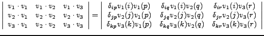
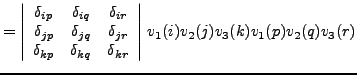
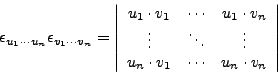
The determinant of a square matrix ![]() of
dimension
of
dimension ![]() is given by
is given by
 :
:
    Symbols a,b,c,d;
    CFunction M;
    Indices i,j;
    Local det = e_(1,2) * e_(i,j) * M(1,i) * M(2,j);
    contract;
    id M(1,1) = a;
    id M(1,2) = b;
    id M(2,1) = c;
    id M(2,2) = d;
    Print;
    .end

   det =
      a*d - b*c;
At first sight, it may look superfluous to put in the local expression
to the front e_(1,2), which is by definition equal to 1. However,
FORM first uses it in the contraction of Levi-Civita tensors, and in this
way, the determinant comes out in explicit form.
In the above example we use the most important command in FORM, viz., the
identify statement id. An
identification is a substitution or replacement. Here we do a straightforward
replacement of matrix elements by their (symbolic) values. As we shall see
in the next chapter, more general patterns are possible in FORM.
For vectors
![]() , the Gram determinant is defined
as the determinant of the matrix
, the Gram determinant is defined
as the determinant of the matrix ![]() with matrix coefficients
with matrix coefficients ![]() equal to
equal to ![]() (the inner product of vectors
(the inner product of vectors ![]() and
and ![]() ).
FORM is the ultimate program for computing such determinants.
First we show how to compute them for
).
FORM is the ultimate program for computing such determinants.
First we show how to compute them for ![]() and
and ![]() with the help of the
Levi-Civita tensor.
with the help of the
Levi-Civita tensor.
    Vectors v1,v2,v3;
    Local G2 = e_(v1,v2)^2;
    Local G3 = e_(v1,v2,v3)^2;
    contract;
    Print;
    .end

   G2 =
      v1.v1*v2.v2 - v1.v2^2;

   G3 =
      v1.v1*v2.v2*v3.v3 - v1.v1*v2.v3^2 + 2*v1.v2*v1.v3*v2.v3 - v1.v2^2*v3.v3
       - v1.v3^2*v2.v2;
To understand the above example, it suffices to recall the definition of
Levi-Civita tensors, the Einstein summation convention, and the SCHOONSCHIP
notation. Let us show this for
![]()
To illustrate that FORM is indeed a very powerful symbol cruncher, let us compute a large Gram determinant of 10 vectors. Actually we only compute the number of terms in the output, because we throw the output away after the program has finished. The computation has been done on a Pentium 166Mhz PC with 16 MB RAM. As you can see, the computation takes less than 9 minutes. If you do the same computation with a general purpose system like Maple or Mathematica on this type of computer, your machine is going to crash or the computation takes basically forever. During the FORM computation many runtime statistics appear, but we have omitted most of them in the printout below.
    AutoDeclare Vector v;
    On statistics;
    Local G10 = e_(v1,...,v10)^2;
    contract;
    .end

Time =       0.60 sec    Generated terms =       6572
              G10      1 Terms left      =       3550
                         Bytes used      =     144066

Time =       0.93 sec    Generated terms =      13043
              G10      1 Terms left      =       8611
                         Bytes used      =     340904

Time =       1.48 sec    Generated terms =      19562
              G10      1 Terms left      =      13910
                         Bytes used      =     538524

                       :
                       :
                       :

Time =     283.00 sec    Generated terms =    3628800
              G10      1 Terms left      =    3075840
                         Bytes used      =  107001398

Time =     283.60 sec
              G10        Terms active    =    3070880
                         Bytes used      =  106917432

Time =     521.78 sec    Generated terms =    3628800
              G10        Terms in output =    1436714
                         Bytes used      =   50113622
Brute force calculation of a 10 by 10 determinant
generates
For us, the declaration and the definition in the above FORM program are interesting, too. The statement
AutoDeclare Vector v;
has the effect that all undeclared variables starting with the character
v will be automatically declared as vectors. In other words,
AutoDeclare makes generic declarations and makes lengthy
declarations in many cases unnecessary.
In the AutoDeclare statement, like in any declaration, you can
limit the maximum power of symbols. For example,
AutoDeclare Symbol x(:3);
makes all undeclared variables starting with the character x
symbols with maximum power of 3.
The three dots operator ... is used in the above FORM program
to generate a sequence of indices:
i1,...,i10 evaluates to
i1,i2,i3,i4,i5,i6,i7,i8,i9,i10.
This is an example of the following more general rule:
x1-...+x6 evaluates to x1-x2+x3-x4+x5-x6.
Another more general example of using the ... operator is the
following: <f1(i1)>*...*<f4(i4)> evaluates to
f1(i1)*f2(i2)*f3(i3)*f4(i4).
This is an example of the following more general rule:
<f4(i2,i6)>*...*<f1(i5,i3)>
evaluates to
f4(i2,i6)*f3(i3,i5)*f2(i4,i4)*f1(i5,i3).
There exist a third delta function, denoted by ![]() and
in FORM by
and
in FORM by dd_, which is totally symmetric and formally equal to a
sum of products of Kronecker deltas.
dd_ generates its terms, it takes symmetries due to
identical arguments into account. Hence, the evaluation of
dd_(v,v,v,v), where v is a vector, generates directly only one
term, viz., v.v, with coefficient 3. This coefficient has a
combinatorial meaning in graph theory: it equals the number of ways
a graph with only one vertex of degree 4 can be realized.
Let us linger upon the application of the function dd_ in graph theory.
First, we associate with vertices ![]() ,
, ![]() ,
, ![]() in a graph
in a graph
![]() vectors
vectors ![]() ,
, ![]() ,
, ![]() , and with edges in the graph, say
, and with edges in the graph, say
![]() and
and ![]() , inner products
, inner products ![]() and
and ![]() .
The latter inner product represents a loop at vertex
.
The latter inner product represents a loop at vertex ![]() , also called
a self-loop at vertex
, also called
a self-loop at vertex ![]() .
For a vertex
.
For a vertex ![]() in a graph the degree of
in a graph the degree of ![]() , denoted by deg(
, denoted by deg(![]() ),
is the number of edges that are incident with
),
is the number of edges that are incident with ![]() . A self-loop is considered
as two incident edges. In the vector notation deg(
. A self-loop is considered
as two incident edges. In the vector notation deg(![]() ) equals the number of
inner products that contain vector
) equals the number of
inner products that contain vector ![]() . A well-known problem in graph theory
is to decide whether a given sequence of nonnegative integers can be
realized as the degrees of the vertices of a graph, and if so, how many
graphs are possible and in how many ways each graph can be realized.
The vector notation for graphs and the FORM function
. A well-known problem in graph theory
is to decide whether a given sequence of nonnegative integers can be
realized as the degrees of the vertices of a graph, and if so, how many
graphs are possible and in how many ways each graph can be realized.
The vector notation for graphs and the FORM function dd_ are
particularly convenient for studying this problem because of automatic
contraction in FORM. The following small example gives the idea:
for two vectors v1 and v2, the formula
dd_(v1,v1,v2,v2) = v1.v1*v2.v2 + 2*v1.v2^2
v1, v2
and each vertex having one self-loop, and that we can construct in two ways a
graph with two edges going from one vertex to the other.
Similarly, the expression dd_(v1,v1,v2,v3) has to do with the
graphs consisting of three nodes, labeled v1, v2 and v3,
and with prescribed degrees deg(v1)=2, deg(v1)=deg(v2)=1.
The formula
dd_(v1,v1,v2,v3) = v1.v1*v2.v3 + 2*v1.v2*v1.v3
v1 having a self-loop and
with an edge connecting the other two vertices, and that there exists a
graph with two edges connecting vertex v1 with the other two vertices,
which can be constructed in two ways.
In general, the expression dd_(
![]()
)
has to do with the graphs consisting of ![]() edges and with prescribed
degrees of the vertices. A vertex
edges and with prescribed
degrees of the vertices. A vertex ![]() occurs
occurs ![]() times as argument in the
function call of
times as argument in the
function call of dd_ if deg(![]() )=
)=![]() .
Each term in the result of the function call corresponds with a graph with
the prescribed degrees. The coefficient of a term tells us in how many ways
the graph represented by the term can be constructed.
The following FORM session shows that 18 graphs can be made
with degree sequence 3,3,3,1. Three of these graphs are loop-free, i.e., have
no self-loops, and they are isomorphic. There exists no loop-free graph
without a multiple edge.
.
Each term in the result of the function call corresponds with a graph with
the prescribed degrees. The coefficient of a term tells us in how many ways
the graph represented by the term can be constructed.
The following FORM session shows that 18 graphs can be made
with degree sequence 3,3,3,1. Three of these graphs are loop-free, i.e., have
no self-loops, and they are isomorphic. There exists no loop-free graph
without a multiple edge.
    AutoDeclare Vector v;
    On Statistics;
    Local F = dd_(v1,v1,v1,v2,v2,v2,v3,v3,v3,v4);
    Print +s F;
    .sort

Time =       0.02 sec    Generated terms =         18
                F        Terms in output =         18
                         Bytes used      =        570

   F =
       + 27*v1.v1*v1.v2*v2.v2*v3.v3*v3.v4
       + 54*v1.v1*v1.v2*v2.v3*v2.v4*v3.v3
       + 54*v1.v1*v1.v2*v2.v3^2*v3.v4
       + 54*v1.v1*v1.v3*v2.v2*v2.v3*v3.v4
       + 27*v1.v1*v1.v3*v2.v2*v2.v4*v3.v3
       + 54*v1.v1*v1.v3*v2.v3^2*v2.v4
       + 27*v1.v1*v1.v4*v2.v2*v2.v3*v3.v3
       + 18*v1.v1*v1.v4*v2.v3^3
       + 54*v1.v2*v1.v3*v1.v4*v2.v2*v3.v3
       + 108*v1.v2*v1.v3*v1.v4*v2.v3^2
       + 54*v1.v2*v1.v3^2*v2.v2*v3.v4
       + 108*v1.v2*v1.v3^2*v2.v3*v2.v4
       + 108*v1.v2^2*v1.v3*v2.v3*v3.v4
       + 54*v1.v2^2*v1.v3*v2.v4*v3.v3
       + 54*v1.v2^2*v1.v4*v2.v3*v3.v3
       + 18*v1.v2^3*v3.v3*v3.v4
       + 54*v1.v3^2*v1.v4*v2.v2*v2.v3
       + 18*v1.v3^3*v2.v2*v2.v4
      ;

    * only loop-free graphs
    Off Statistics;
    id v1.v1 = 0;
    id v2.v2 = 0;
    id v3.v3 = 0;
    Print +s F;
    .sort

   F =
       + 108*v1.v2*v1.v3*v1.v4*v2.v3^2
       + 108*v1.v2*v1.v3^2*v2.v3*v2.v4
       + 108*v1.v2^2*v1.v3*v2.v3*v3.v4
      ;

    * no multiple edges
    id v1.v2^2 = 0;
    id v1.v3^2 = 0;
    id v2.v3^2 = 0;
    Print +s F;
    .end

   F = 0;
The conditions for ``loop-free'' and ``no multiple edges'' can
be expressed much shorter in FORM than was done in the above session.
As we shall see in the next chapter id v?.v? = 0 is short notation
for saying that every inner product of a vector with itself equals zero.
id u?.v?^2 = 0 is short notation for saying that no inner product
with exponent 2 occurs. Hence, the following session proves that there exists
only one loop-free graph without multiple edges and with degree sequence
5,5,4,3,3,2.
    AutoDeclare Vector v;
    Local F = dd_(v1,v1,v1,v1,v1,
                  v2,v2,v2,v2,v2,
                  v3,v3,v3,v3,
                  v4,v4,v4,
                  v5,v5,v5,
                  v6,v6);
    id v?.v?=0;     * loop-free
    id v1?.v2?^2=0; * no multiple edges
    Format 65;
    Print F;
    .end

   F =
      24883200*v1.v2*v1.v3*v1.v4*v1.v5*v1.v6*v2.v3*v2.v4*v2.v5*
      v2.v6*v3.v4*v3.v5;
The third last command Format 65 is used to control the width of
the output: 65 columns at most.
The expression corresponds with the following graph:
 .
.
sump_.
It works like the regular function sum_, except
that the last argument is not the sump_(i,0,10,x) evaluates
to the series expansion of
Use the function sump_ to compose the
expression
 ,
and write it as a polynomial in
,
and write it as a polynomial in ![]() .
.
 , but throw away all powers of degree 4 and higher.
where there are ![]() lines constructed with the
lines constructed with the ![]() , and
, and ![]() lines constructed
with the
lines constructed
with the ![]() .
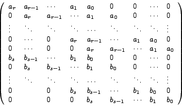
The resultant of
.
The resultant of ![]() and
and ![]() , denoted by
, denoted by
![]() ,
or
,
or
![]() if there has to be a
variable
if there has to be a
variable ![]() , is the determinant of the Sylvester matrix.
The importance of the resultant lies in the following theorem.
, is the determinant of the Sylvester matrix.
The importance of the resultant lies in the following theorem.
    AutoDeclare Vectors u,v;
    Symbol a,b,c,d;
    Local det = e_(u1,u2)*e_(v1,v2);
    contract;
    id u1.v1 = a;
    id u1.v2 = b;
    id u2.v1 = c;
    id u2.v2 = d;
    Print;
    .end

   det =
      a*d - b*c;
dd_ in graph theoretical enumeration problems.
dd_.
Many operations in a FORM program are in the form of substitutions:
replacing one pattern by another one. The identify or shortly
id statement does this in various ways. In the previous chapter
we have already seen how it can be used for a straightforward substitution.
In fact, it will only be a one-time substitution as the following example illustrates.
    Symbol x;
    Local expr = x + 1/x;
    id x = x+1;
    Print;
    .sort

   expr =
      1 + x^-1 + x;

    id x = x+1;
    Print;
    .end

   expr =
      2 + x^-1 + x;
The replacement rule
id statement will never act on its own
right hand side. It will only take any natural power of
Another rather straightforward substitution is the replacement of an
integer power of a symbol (exponent ![]() is forbidden) or of products of such
powers. There will be as many substitutions as possible, e.g., the
replacement
is forbidden) or of products of such
powers. There will be as many substitutions as possible, e.g., the
replacement
![]() transforms
transforms ![]() into
into ![]() . Examples of
substitution:
. Examples of
substitution:
    Symbols x,y,z,k;
    Local expr = sum_(k,-2,5,x^k);
    Print;
    .sort

   expr =
      1 + x^-2 + x^-1 + x + x^2 + x^3 + x^4 + x^5;

    id x^2 = y;
    Print;
    .sort

   expr =
      1 + x^-2 + x^-1 + x*y + x*y^2 + x + y + y^2;

    id x*y = z;
    Print;
    .sort

   expr =
      1 + x^-2 + x^-1 + x + y*z + y + y^2 + z;

    id 1/x = z^2;
    Print;
    .end

   expr =
      1 + x + y*z + y + y^2 + z + z^2 + z^4;
Expressions can be used in the right-hand side of statement; so, also
in the id statement. FORM uses the definitions of the
expressions as they are present at the start of the module in which the
id statement is applied.
An example:
    Symbol x,y;
    Local expr = x*y;
    id x = expr;
    Print;
    .sort

   expr =
      x*y^2;

    id x = expr;
    id x = expr;
    Print;
    .end

   expr =
      x*y^6;
To summarize straightforward substitution: the left-hand side of the
replacement rule may be a product of a few factors with exponents, but
may not contain a numerical factor, or be a sum of terms.
For example, id 2*x*y=z and id x+y=z are invalid
statements. The right-hand side only has to be a valid expression.
Often one wants to apply a substitution rule repeatedly until it causes no
further change anymore. This is accomplished by surrounding the command
by repeat and endrepeat.
Three examples will do. The first example is a computation of a
Fibonacci number. The last two examples come from quantum mechanics:
working out the commutation relations of position and momentum operator,
and working out a product of Pauli matrices.
In the following example we shall use a replacement rule to compute the
nineteenth Fibonacci number ![]() . Recall that the Fibonacci numbers
. Recall that the Fibonacci numbers
![]() are recursively defined as
are recursively defined as
    Symbol x;
    Local Fibonacci19 = x^18;
    repeat;
      id x^2 = x + 1;
    endrepeat;
    id x = 1;
    Print;
    .end

   Fibonacci19 =
      4181;
We use the commutation relation
![]() between position operator
between position operator ![]() and momentum operator
and momentum operator ![]() repeatedly to
work out the commutation relation
repeatedly to
work out the commutation relation
![]() for the Hamiltonian
for the Hamiltonian
 .
In the example we shall use the built-in variable
.
In the example we shall use the built-in variable i_ for
the complex unit ![]() .
The mass
.
The mass ![]() and Planck's constant
and Planck's constant ![]() (
(
![]() )
are declared as symbols as they commute with everything else; The Hamiltonian,
position, and momentum operators are declared as noncommuting
functions.
)
are declared as symbols as they commute with everything else; The Hamiltonian,
position, and momentum operators are declared as noncommuting
functions.
    Symbols hbar,m;
    Functions x,p,H;
    Local [H,x] = H*x - x*H;
    id H = p^2/(2*m);
    Print;
    .sort

   [H,x] =
       - 1/2*x*p*p*m^-1 + 1/2*p*p*x*m^-1;

    repeat;
      id x*p = p*x + hbar*i_;
    endrepeat;
    Print;
    .end

   [H,x] =
       - p*i_*hbar*m^-1;
In no time, FORM gives the answer
![$\displaystyle [H,x]=-\frac{h\hskip-.2em\llap{\protect\rule[1.1ex]{.325em}
{.1ex}}\hskip.2em\,i}{m}\,p$](img174.png) .
.
We consider the algebra generated by
![]() , and
, and ![]() satisfying the relations
satisfying the relations
    Function s;
    Index k;
    Dimension 3;
    Local [s(1)*s(2)] = i_*e_(1,2,3)*e_(1,2,k)*s(k);
    Local [s(1)*s(3)] = i_*e_(1,2,3)*e_(1,3,k)*s(k);
    Local [s(2)*s(3)] = i_*e_(1,2,3)*e_(2,3,k)*s(k);
    contract;
    Print;
    .sort

   [s(1)*s(2)] =
      s(3)*i_;

   [s(1)*s(3)] =
       - s(2)*i_;

   [s(2)*s(3)] =
      s(1)*i_;

    Local F = ( s(1)*s(2) + s(1) + s(2) + s(3) )^4;
    repeat;
      id s(2)*s(1) = -s(1)*s(2);
      id s(3)*s(1) = -s(1)*s(3);
      id s(3)*s(2) = -s(2)*s(3);
      id s(1)*s(2) = [s(1)*s(2)];
      id s(1)*s(3) = [s(1)*s(3)];
      id s(2)*s(3) = [s(2)*s(3)];
      id s(1)^2 = 1;
      id s(2)^2 = 1;
      id s(3)^2 = 1;
    endrepeat;
    Print F;
    .end

   F =
      8*i_;
In the first module, we let FORM compute various products of Pauli matrices.
These results are used in the second module to work out formulas.
 . Express
 into
into


 .
.
 do not form a
Lie algebra.
do not form a
Lie algebra.
In the previous section we have looked at straightforward substitution via the
id statement: a symbol, a power of a symbol, and products of
powers of symbols were replaced by new expressions.
However, very often you do not only want particular objects being
replaced, but actually all objects of a certain type.
For example, if you are interested in integrating polynomials in one
variable ![]() , you do not want to replace
, you do not want to replace ![]() for specific values of
the natural number
for specific values of
the natural number ![]() by
by
![]() , but instead for all
natural numbers. The rest of this chapter will be about such pattern
matching.
, but instead for all
natural numbers. The rest of this chapter will be about such pattern
matching.
A pattern in FORM, also called a wildcard,
is an elegant way of representing the syntactical structure of an
expression. The atomic pattern objects are denoted by a
variable followed by a question mark
and represent one single object. For example,
if x is a symbol, then x? will represent any symbol and
x?^2 will represent any square of a symbol. If p(i) represents
the vector p with index i, then p(i?) represents
the vector p with any index, p?(i) represents any vector with
index i, and p?(i?) represents any vector with any index.
And so on.
Because patterns are in general not restricted to single objects
they can become rather complicated. For example, x * y^n? * f(i,g?(i))
is a valid FORM pattern. In case x, y, i, n are
symbols, and f, g are functions, the above pattern represents
a product of x, any integer power of y, and a function
f of which the first argument is equal to i and the second one
is any function with argument i.
One more thing that you have to take into account when dealing
with more complicated patterns: when a wildcard such as x? appears
twice in the left-hand side of an id statement both occurrences have
to match the same argument. For example, for two vectors u and v,
the pattern u?.u? represents any dot product of a vector with itself,
and u?.v? represents any dot product, including the case of
identical vectors in the dot product.
Advice: if you find it difficult to answer right now the exercises below, then work through the examples of the next section and come back to these exercises afterwards. Or try things out in FORM to get the idea.
x, n, explain what the
following patterns mean.
x
1/x
x?
x^n?
x?^n
x?^n?
u, v and the indices i,
j, explain what the
following patterns mean.
u(i)
u(i?)
u?(i)
u?(i?)
u(i?)*v(j?)
u(i?)*v(i?)
u.v?
u?.v?
v?.v?
u?.v?^2
Patterns are used in replacement rules. In this section, we shall give examples that show you how to use wildcards in FORM.
    Symbols x,y,z,n;
    Local F = x^2 + y^3 + 1;
    id x? = z;
    Print;
    .sort

   F =
      1 + z^2 + z^3;

    id z^n? = x;
    Print;
    .sort

   F =
      3*x;

    Local G = F + y^2 + 1;
    id x?^n? = z;
    Print G;
    .end

   G =
      1 + 4*z;
Let us have a closer look at the above session. Because
In the next two examples we shall use replacement rules to compute the
nineteenth Fibonacci number ![]() . Recall that the Fibonacci numbers
. Recall that the Fibonacci numbers
![]() are recursively defined as
are recursively defined as
    Symbols last, secondlast, dummy;
    Function F;
    On statistics;
    Local Fibonacci19 = F(1,1) * dummy^17;
    repeat;
      id F(last?, secondlast?) * dummy = F(last + secondlast, last);
    endrepeat;
    id F(last?, secondlast?) = last;
    Print;
    .end

Time =       0.04 sec    Generated terms =          1
      Fibonacci19        Terms in output =          1
                         Bytes used      =         10

   Fibonacci19 =
      4181;
Three remarks:
dummy^17 and use
a replacement rule that lowers the power of dummy by one.
The repetition stops when no power of dummy is left.
This trick of tagging an expression by a dummy variable to control repetition
or to apply certain operations from left to right or vice versa
in the expression is often used in FORM programs.
id-statement, viz. last? and secondlast?. They both
match any function argument in the call of F. Then, in the right
hand-side of the id-statement, last and secondlast
will be replaced by the matched numbers.
A downward recursion would result in a less efficient program with respect to computing time and number of terms generated.
    Symbols n;
    Function F;
    On statistics;
    Local Fibonacci19 = F(19);
    repeat;
      id F(1) = 1;
      id F(2) = 1;
      id F(n?) = F(n-1) + F(n-2);
    endrepeat;
    Print;
    .end

Time =       6.19 sec    Generated terms =       4181
      Fibonacci19        Terms in output =          1
                         Bytes used      =         10

   Fibonacci19 =
      4181;
Differentiation of bivariate polynomials, say computing the derivative
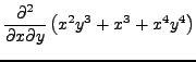 , can be done as follows in FORM.
    Symbols x,y,m,n;
    Local P = x^2*y^3 + x^3 + x^4*y^4;
    Print;
    .sort

   P =
      x^2*y^3 + x^3 + x^4*y^4;

    id  x^m? * y^n? = m*x^(m-1) * n*y^(n-1);
    Print;
    .end

   P =
      6*x*y^2 + 16*x^3*y^3;
An example from vector calculus: given a basis transformation
![]() , a vector
, a vector ![]() in the
in the ![]() -basis defined as
-basis defined as
![]() , and the restriction that the matrices
, and the restriction that the matrices ![]() and
and
![]() are inverses of each other, describe
are inverses of each other, describe ![]() in the
in the ![]() -basis.
-basis.
    Vector x,y;
    Tensors g,a,b;
    Indices i,j,k;
    Local [y(k)] = b(k,x);
    Local [T(i)] = g(i,j) * a(j,k) * [y(k)];
    id a(i?,k?) * b(k?,j?) = d_(i,j);
    Print [T(i)];
    .end

   [Tx(i)] =
      g(i,x);
So, we have proved with FORM that
Let us illustrate the rules about repeated wildcards
for a user-defined Levi-Civita tensor eps
and a user-defined Kronecker symbol delta
with various contractions in 3-dimensional space.
    Dimension 3;
    Tensors eps(antisymmetric), delta(symmetric);
    Indices i,j,k,l,m,n;
    *
    * three repeated indices
    *
    Local F1 = eps(i,j,k) * eps(i,j,k);
    id eps(i?,j?,k?) * eps(i?,j?,k?) = 6;
    Print F1;
    .sort

   F1 =
      6;

    *
    * two repeated indices; antisymmetry is applied
    *
    Local F2 = eps(i,j,k) * eps(i,j,l);
    id eps(i?,j?,k?) * eps(i?,j?,l?) = delta(k,l);
    Print F2;
    .sort

   F2 =
      delta(k,l);

    *
    * one repeated index
    *
    Local F3 = eps(i,j,k) * eps(i,l,m);
    id eps(i?,j?,k?) * eps(i?,l?,m?) = delta(j,l) * delta(k,m) -
                                       delta(j,k) * delta(l,m);
    Print F3;
    .sort

   F3 =
       - delta(j,k)*delta(l,m) + delta(j,l)*delta(k,m);

    *
    * no repeated index; only antisymmetry is applied
    *
    Local F4 = eps(i,j,k) * eps(n,m,l);
    id eps(i?,j?,k?) * eps(l?,m?,n?) = eps(i,j,k) * eps(l,m,n);
    Print F4;
    .end

   F4 =
       - eps(i,j,k)*eps(l,m,n);

 .
.
For functions there are basically four types of wildcarding:
We have already seen examples of such wildcarding in the previous
section. But let us look at another one. Suppose that we want to
implement in FORM the simplification
![]() ,
and apply it to
,
and apply it to ![]() ,
,
![]() , and
, and
![]() .
.
    Symbols a,b,x,y;
    CFunction sqrt;
    Local F1 = a * sqrt(b);
    Local F2 = sqrt(2) * sqrt(b);
    Local F3 = sqrt(sqrt(a)+1) * sqrt(sqrt(a)-1);
    id x? * sqrt(y?) = sqrt(x^2*y);
    Print;
    .sort

   F1 =
      sqrt(a^2*b);

   F2 =
      sqrt(2)*sqrt(b);

   F3 =
      sqrt( - 1 + sqrt(a))*sqrt(1 + sqrt(a));

    repeat;
      id sqrt(x?) * sqrt(y?) = sqrt(x*y);
    endrepeat;
    id sqrt(4) = 2;
    Print F2,F3;
    .sort

   F2 =
      sqrt(2*b);

   F3 =
      sqrt( - 1 + sqrt(a)^2);

    argument;
      id sqrt(x?) * sqrt(x?) = x;
    endargument;
    Print F3;
    .end

   F3 =
      sqrt( - 1 + a);
As you see the pattern x? * sqrt(y?) only matches the first formula;
the factors sqrt(sqrt(a)+1) and sqrt(2) are no symbols.
If you specify a pattern sqrt(x?) * sqrt(y?), then these
expressions match.
Note that in this case the wildcard may match a whole composite expression.
Alas, the identification has not replaced the product of square roots
inside the last formula. For efficiency reason, the rule in FORM is that
substitutions are not executed inside the arguments of functions.
Therefore FORM has a special environment that
allows manipulation of function arguments. This environment is indicated by
the keywords argument and endargument, as shown in the third
module in the above program.
argument environments can be nested. The next example illustrates this.
    CFunction f;
    Symbols x,y;
    Local expr = f(x,f(x));
    id x=y;
    Print;
    .sort

   expr =
      f(x,f(x));

    argument;
      id x=y;
    endargument;
    Print;
    .sort

   expr =
      f(y,f(x));

    argument;
      argument;
        id x?=y^2;
      endargument;
    endargument;
    Print;
    .end

   expr =
      f(y,f(y^2));
There is nothing special about wildcards of functions or about the combination of this and the previous type of wildcarding. We give one example that shows all.
    Symbols x,y,z;
    CFunctions f,g,h;
    Local expr1 = f(x) + g(y);
    id f?(x) = h(x);
    Print;
    .sort;

   expr1 =
      g(y) + h(x);

    Local expr2 = f(x) + g(y);
    id f?(x?) = z;
    Print expr2;
    .sort;

   expr2 =
      2*z;

    Local expr3 = f(x+y) + f(x,y);
    id f?(x?) = z;
    Print expr3;
    .end

   expr3 =
      z + f(x,y);
We added the last module to illustrate once more that a symbol can match
as a function argument a whole expression. But from this example, you also
see that it can only match one argument and not more. To achieve this we
need a special kind of wildcard that refers to a group of arguments in a
function. This is the topic of the next subsection.
The wildcarding in FORM allows you to refer to a group of parameters.
For example, the id statement in the example below uses
a variable that starts with a question mark
to represent any sequence of adjacent arguments in a function call.
We call this an argument sequence wildcard.
    Symbols x,y;
    CFunctions f,g;
    Local F = f(x,x,x) + f;
    id f(?a) = g(0,?a,0,?a,0);
    Print;
    .end

   F =
      g(0,x,x,x,0,x,x,x,0) + g(0,0,0);
The variables ?a in the right hand side of the identify statement
refer to the match of the wildcard.
A few remarks:
f is a function and x,
y are symbols, then the pattern f?(x,?a)*f?(y,?b) matches
the product of any function which starts with x and the same
function that starts with y. The pattern f?(?a, x, ?b) matches
any function that has an argument x.
    Symbols w,x,y,z;
    Indices W,X,Y,Z;
    CFunction F;
    Tensor S(symmetric), C(cyclic);
    Local expr = F(x,y,z) + S(X,Y,Z) + C(X,Y,Z);
    id F(?a,w?,?b) = F(w,0,?a,0,?b);
    id S(?a,W?,?b) = S(W,0,?a,0,?b);
    id C(?a,W?,?b) = C(W,0,?a,0,?b);
    Print;
    .end

   expr =
      F(z,0,x,y,0) + S(X,Y,Z) + C(0,0,Y,Z,X);
Let us illustrate the wildcarding with argument fields by another example
taken from tensor calculus. We consider the metric tensor ![]() , and the Riemann tensor
and Ricci tensor denoted by
, and the Riemann tensor
and Ricci tensor denoted by ![]() . We show how you can implement in FORM the contractions
. We show how you can implement in FORM the contractions
![]() and
and
![]() .
It will also be an illustration of how one can compute with upper
(contravariant) and lower (covariant) indices in
FORM.
.
It will also be an illustration of how one can compute with upper
(contravariant) and lower (covariant) indices in
FORM.
    Tensors g,R;
    Indices i,j,k,l,m,n,low,up;
    Local T1 = g(i,low,j,up) * R(j,low,k,low);
    Local T2 = g(i,up,j,up) * R(i,low,k,low,j,low,l,low);
    id g(i?,low,j?,up) * R?(?a,j?,low,?b) = R(?a,i,low,?b);
    id g(i?, up,j?,up) * R?(?a,i?,low,?b,j?,low,?c) = R(?a,?b,?c);
    id g(i?, up,j?,up) * R?(?a,j?,low,?b,i?,low,?c) = R(?a,?b,?c);
    Print;
    .end

   T1 =
      R(i,low,k,low);

   T2 =
      R(k,low,l,low);
As you see, we simply keep track of the type of the index by putting next
to the index in the function call a special index low or up,
and we distinguish the indices by type in the identifications.
The third identify statement has only been added for
the general case where repeated indices may be interchanged.
Of course, the above implementation of upper and lower indices is
somewhat cumbersome. So let us introduce a shorter notation
such as U(i) and L(j) for an upper index i and lower
index j, respectively. The example now looks as follows:
    Functions g,R,L,U;
    Indices i,j,k,l,m,n;
    Local T1 = g(L(i),U(j)) * R(L(j),L(k));
    Local T2 = g(U(i),U(j)) * R(L(i),L(k),L(j),L(l));
    id g(L(i?),U(j?)) * R?(?a,L(j?),?b) = R(?a,L(i),?b);
    id g(U(i?),U(j?)) * R?(?a,L(i?),?b,L(j?),?c) = R(?a,?b,?c);
    id g(U(i?),U(j?)) * R?(?a,L(j?),?b,L(i?),?c) = R(?a,?b,?c);
    Print;
    .end

   T1 =
      R(L(i),L(k));

   T2 =
      R(L(k),L(l));
It works! But it is good to realize that we rely on certain aspects of
FORM.
Firstly, note that there is ambiguity in the matching of the pattern
R?(?a,L(j?),?b) with the expression R(L(j),L(k)): should the
first question mark variable be an empty argument sequence or should the second
question mark variable match an empty statement. In the latter case,
the first identification in the above example will have no match.
Apparently FORM searches
until it finds a match. Secondly, note that a nested wildcarding for
functions is used. Although FORM allows this, for efficiency reasons,
it will in general not try out all possible matchings. Once it has found
a match, it will stop looking for further matches. Apparently we were
lucky in the wildcarding of our example: FORM selected the correct pattern match for getting
the work done.
By denesting you can get more control about the wildcarding of nested functions. Below we show you how to do this in our example.
    Functions g,R,L,U;
    Indices i,j,k,l,m,n,low,up;
    Local T1 = g(L(i),U(j)) * R(L(j),L(k));
    Local T2 = g(U(i),U(j)) * R(L(i),L(k),L(j),L(l));
    *
    * denest functions
    *
    repeat;
      id R?(?a,L(i?),?b) = R(?a,i,low,?b);
      id R?(?a,U(i?),?b) = R(?a,i,up,?b);
    endrepeat;
    *
    * apply rules
    *
    id g(i?,low,j?,up) * R?(?a,j?,low,?b) = R(?a,i,low,?b);
    id g(i?, up,j?,up) * R?(?a,i?,low,?b,j?,low,?c) = R(?a,?b,?c);
    id g(i?, up,j?,up) * R?(?a,j?,low,?b,i?,low,?c) = R(?a,?b,?c);
    *
    * back to original notation
    *
    repeat;
      id R?(?a,i?,low,?b) = R(?a,L(i),?b);
      id R?(?a,i?, up,?b) = R(?a,L(i),?b);
    endrepeat;
    *
    * Print the results
    *
    Print;
    .end

   T1 =
      R(L(i),L(k));

   T2 =
      R(L(k),L(l));
In the next section, we shall show another way of handling upper and lower
indices which does not lead to two representations of the same mathematical
object.
 , and that a covariant tensor
 .
.
ToVector command replaces a tensor into a product
of vector components. For example,
ToVector t,v replaces
t(m1,m2,m3) by v(m1)*v(m2)*v(m3). Use id statements
to get the same job done.
 for
for
We shall use as metric tensor ![]() and its inverse
and its inverse ![]() for special relativity the one with sign convention
for special relativity the one with sign convention
![]() and
and
![]() , for
, for ![]() .
Then the full contravariant form
.
Then the full contravariant form ![]() is
is
The pattern matching we have seen thus far involved wildcards that would match any variable of proper type. Furthermore, no restrictions on the replacement rules have been made. In this section, we shall see how to get more control over the wildcards and replacements. The last three subsections will contain ``real world'' examples of differentiation of functions, tensor calculus with upper and lower indices, and computation with gamma matrices.
One of the types of variables in FORM is ``set'' or ``array''. An example that explains the data type:
    Symbol a1,a2;
    Set a:a1,a2;
    Local F = a[1] + a[2];
    Print;
    .end

   F =
      a1 + a2;
As you see, FORM assumes that sets or arrays start with index 1.
Furthermore, sets are homogeneous objects, i.e., elements of sets must be
of the same type.
Sets are mostly used in wildcarding.
    Symbols a,b,c,x;
    Local F = a + b + c;
    id x?{b,c} = 3;
    Print;
    .end

   F =
      6 + a;
x? would mean ``any symbol'', whereas in our example
we restrict the symbols to the set ?!.
    Symbols a,b,c,x;
    Local F = a + b + c;
    id x?!{b,c} = 3;
    Print;
    .end

   F =
      3 + b + c;
We called sets also arrays because wildcarding sets behave like these.
    Symbols a1,a2,b1,b2,x,n;
    Function f;
    Set a : a1,a2;
    Set b : b1,b2;
    Local F = a[1] + a[2];
    id x?a[n] = b[n] + f(n);
    Print;
    .end

   F =
      b1 + b2 + f(1) + f(2);
In the above example, x must belong to the set a, and
n becomes the number of the element in the set to which
x matches. The same number is used at the right hand side of
the identity. However, no arithmetic can be done with n.
There exists a shortcut for changing names of set elements.
    Symbols a1,a2,b1,b2,x,n;
    Set a : a1,a2;
    Set b : b1,b2;
    Local F = a[1] + a[2];
    id x?a?b = x;
    Print;
    .end

   F =
      b1 + b2;
Here, the identity statement reads as follows: x must
belong to the set a, and in the right hand side each occurrence of
x will be replaced by the corresponding element of the set b.
The built-in sets in FORM are listed below. As all built-in objects, they end with an underscore.
| Set | Meaning: set of |
even_ |
even integers |
fixed_ |
fixed indices |
index_ |
all indices |
int_ |
integers |
neg_ |
negative integers |
neg0_ |
nonpositive integers |
number_ |
all rational numbers |
odd_ |
odd integers |
pos_ |
positive integers |
pos0_ |
nonnegative integers |
symbol_ |
only symbols |
Intervals can be specified as so-called ranged sets.
{>=-3,<5, {<10}, and {>=2} denote ![]() ,
,
![]() , and
, and ![]() , respectively.
, respectively.
With the built-in sets and the range sets you can restrict wildcards to some infinite sets as is shown in the next example.
    Symbols x,n;
    Local F = sum_( n, -3, 3, x^n );
    Print;
    .sort

   F =
      1 + x^-3 + x^-2 + x^-1 + x + x^2 + x^3;

    id x^n?pos_ = 0;
    Print;
    .sort

   F =
      1 + x^-3 + x^-2 + x^-1;

    id x^n?!even_ = 0;
    Print;
    .end

   F =
      1 + x^-2;
Here, we replace first all positive powers of x by zero, and hereafter
we remove all powers with odd exponent.
When you create a couple of identifications, there may be a conflict of
what rule to apply first. In FORM, you can influence the applicability
of an identification by options. One of the options is
select.
It is followed by the names of one or more sets of symbols, functions,
vectors, or indices. No built-in sets are allowed in the select
statement.
The replacement rule will only be applied if after the matching of the
left-hand side no elements of the mentioned sets are left anywhere in the
term. An example explains it better.
    Symbols a,b,c,d;
    Functions f,g;
    Index i;
    Set bcSet: b,c;
    Local F1 = a*b*c;
    id select bcSet a*b = b^2;
    id select bcSet a*b*c = b^2*c^2;
    Print;
    .sort

   F1 =
      b^2*c^2;

    Local F2 = f(i,a)*b + f(i,b)*c;
    id select bcSet c?=g(d);
    Print;
    .end

   F1 =
      b^2*c^2;

   F2 =
      f(i,a)*g(d) + f(i,b)*c;
In the above example, the first replacement rule is not applied
because after matching ab in the product abc the
element c of the set {b,c} is left behind. The second
replacement rules matches F1 and will be applied.
The third replacement rule is applied to first term of expression
F2 only. After matching a symbol in the second term of F2
there is still an element of the set F1 when one tries to apply the replacement rule.
There are more options to identify statements in FORM. Below we tabulate them and we illustrate the use of some of them.
| Option | Meaning |
disorder |
substitution in non-commutative algebra |
ifmatch |
if there is a match, jump to a label after substitution |
many |
multiple matches |
multi |
single match with multiplicity |
once |
single match |
only |
exact match |
select |
match with no selected symbols, functions, |
| vectors, or indices left |
    Symbols a,b,x,y,z;
    Local F0 = (x+y)^4;
    Print F0;
    .sort

   F0 =
      4*x*y^3 + 6*x^2*y^2 + 4*x^3*y + x^4 + y^4;

    Local F1 = (x+y)^4;
    id once x = z;
    Print F1;
    .sort

   F1 =
      6*x*y^2*z + 4*x^2*y*z + x^3*z + 4*y^3*z + y^4;

    Local F2 = (x+y)^4;
    id x*y = z;
    Print F2;
    .sort

   F2 =
      4*x^2*z + x^4 + 4*y^2*z + y^4 + 6*z^2;

    Local F3 = (x+y)^4;
    id only x*y = z;
    Print F3;
    .sort

   F3 =
      4*x*y^3 + 6*x^2*y^2 + 4*x^3*y + x^4 + y^4;

    Local F4 = (a+b)^2 * (x+y)^2;
    Print F4;
    .sort

   F4 =
      4*a*b*x*y + 2*a*b*x^2 + 2*a*b*y^2 + 2*a^2*x*y + a^2*x^2 + a^2*y^2 + 2*
      b^2*x*y + b^2*x^2 + b^2*y^2;

    id multi x?*y? = z;
    Print F4;
    .end

   F4 =
      2*a*y*z + 2*b*y*z + 4*x*y*z + 2*x^2*z + 2*y^2*z + 4*z^2;
The normal rule for pattern matching in FORM is that the pattern
is taken out as many times as possible before inserting the right-hand
side (the most important exception
is a wildcard power). No second attempt of pattern matching is made.
In the first identification in the above example, the option once
overrules the general behavior of the system: only one single
match of a pattern is attempted. By the way, the default is
many. The next two identifications in the example are
replacements
only implies that the match must be exact.
Finally, the option multi is used: it
means a single matching with multiplicity. In the given example, it means
that when it is applied to the term
The ifmatch option is mostly used in cases where there is a long
list of substitutions, but applying them all at once would make the
substitution tree too complicated. Below we only give a simple example to
illustrate the syntax and semantics of the statement. We remove
from a polynomial in two variables ![]() and
and ![]() all monomials in
all monomials in ![]() and
replace
and
replace x by the symbol z.
    Symbols x,y,z;
    Local F = x^2*y + y + 1;
    id ifmatch->1 x=z;
      id y=0;
    label 1;
    Print;
    .end

   F =
      1 + y*z^2;
The statement id ifmatch->1, x=z; will lead to a jump to label 1
if there is a match and after the substitution has been made.
Logically the above program is equivalent to
    Symbols x,y,z;
    Local F = x^2*y + y + 1;
    if ( match(x) );
      id x = z;
    else;
      id y=0;
    endif;
    Print;
    .end

   F =
      1 + y*z^2;
Such a nesting of if-statements becomes rather impractical when many
statements are involved. Moreover in this setup the matching has to be
done twice, while the ifmatch construction involves only a single
pattern matching.
We shall describe the option disorder with an example from Dirac
algebra in dimension 4. The Dirac gamma matrices ![]() ,
, ![]() ,
,
![]() , and
, and ![]() have the properties
have the properties
    Functions g3,...,g0,g,h;
    Local [g5] = i_ * g0 * g1 * g2 * g3;
    Local [g5^2] = [g5]^2;
    Local [g0*g5+g5*g0] = g0 * [g5] + [g5] * g0;
    Local [g1*g5+g5*g1] = g1 * [g5] + [g5] * g1;
    Local [g2*g5+g5*g2] = g2 * [g5] + [g5] * g2;
    Local [g3*g5+g5*g3] = g3 * [g5] + [g5] * g3;
    repeat;
      id g0*g0 = 1;
      id g?*g? = -1;
      id disorder g? * h?= - h * g;
    endrepeat;
    Print;
    .end

   [g5] =
      g0*g1*g2*g3*i_;

   [g5^2] =
      1;

   [g0*g5+g5*g0] = 0;

   [g1*g5+g5*g1] = 0;

   [g2*g5+g5*g2] = 0;

   [g3*g5+g5*g3] = 0;
You may have expected replacement rules like:
id g2 * g1 = -g1 * g2;
id g3 * g1 = -g1 * g3;
id g3 * g2 = -g2 * g3;
id g4 * g1 = -g1 * g4;
id g4 * g2 = -g2 * g4;
id g4 * g3 = -g3 * g4 ;
But this is rather cumbersome. It is much easier to rely on the internal ordering of the functions and to have just one identification like
id g? * h? = - h*gBut when you repeat such a replacement rule, you would get into an infinite loop. To avoid this, the option
disorder has been introduced
in FORM. With this option, the identification is applied when the
normal ordering of terms in the pattern would change the order of the
functions, if they were commuting.
In subsection 2.5.5 we shall discuss in detail how
to compute with gamma matrices in FORM.
By now, you should be able to understand the following more realistic example of differentiation of trigonometric functions.
    Symbols x,y,n;
    CFunctions sin,cos,tan,g;
    Functions [sin], [cos], [tan], [-sin], [1/cos^2], f, dx;
    Set commuting: sin, cos, tan;
    Set noncommuting: [sin], [cos], [tan];
    Set derivative: [cos], [-sin], [1/cos^2];
    *
    Local expr = sin(x)*tan(x) + cos(x);
    *
    id g?commuting?noncommuting(x) = g(x);
    Multiply left dx;
    repeat;
      id dx*g?noncommuting[n](x) = derivative[n](x) + g(x)*dx;
      id [-sin](x) = - [sin](x);
      id [1/cos^2](x) = 1/[cos](x) * 1/[cos](x);
    endrepeat;
    id dx = 0;
    id f?noncommuting?commuting(x) = f(x);
    id 1/f?noncommuting?commuting(x) = 1/f(x);
    *
    Print;
    .end

   expr =
       - sin(x) + cos(x)*tan(x) + 1/(cos(x))/(cos(x))*sin(x);
Now that we know about sets, we can look at another FORM implementation
of contravariant and covariant indices. We consider
the same example as in Section 2.4.3.
Covariant or lower indices like a and b are denoted by
La and Lb, where
the leading L stands for ``lower''. Similarly, contravariant or
upper indices like a and b are denoted by Ua and
Ub,
where the leading U stands for ``upper''. We define two set, viz.,
LU and UL, that enable us to check whether an index appears
twice but of opposite type. This make it easy to define the replacement
rules for raising and lowering indices with the metric tensor as the
example below shows. We will work out the Ricci curvature tensor and
the trace of the metric tensor.
    Tensors g,R,h;
    AutoDeclare Indices U,L;
    Indices i,j,k,l,m;
    Set UL: Ui, Li, Uj, Lj, Uk, Lk, Ul, Ll;
    Set LU: Li, Ui, Lj, Uj, Lk, Uk, Ll, Ul;
    Symbol n;
    *
    Local T1 = g(Li, Uj) * R(Lj, Lk);
    Local T2 = g(Ui, Uj) * R(Li, Lk, Lj, Ll);
    Local T3 = g(Ui, Lj) * R(Li, Uj);
    Local T4 = g(Ui, Lj) * g(Uj, Li);
    *
    repeat;
      id g(?a, i?UL[n], ?b) * h?(?c, j?LU[n], ?d) = h(?a, ?b, ?c, ?d);
      id h?(?a, i?UL[n], ?b, j?LU[n], ?c) = h(?a, ?b, ?c);
    endrepeat;
    *
    Print;
    .end

   T1 =
      R(Li,Lk);

   T2 =
      R(Lk,Ll);

   T3 =
      R;

   T4 =
      g;
No indices in the answers means implicitly that contraction of all
indices took place.
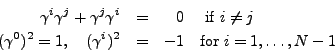
First, we shall implement calculus with ![]() -dimensional
Dirac gamma matrices and pay extra attention to the case
-dimensional
Dirac gamma matrices and pay extra attention to the case ![]() .
Later in this subsection we shall look at the class of gamma matrices
available in FORM and at how to use them to compute traces.
.
Later in this subsection we shall look at the class of gamma matrices
available in FORM and at how to use them to compute traces.
Henceforth, we shall use the Bjorken & Drell metric with indices
running over time-space from 0 to ![]() , and with metric tensor
, and with metric tensor
![]() defined by
defined by ![]() ,
, ![]() , for
, for
![]() , and
, and
![]() , for
, for
![]() . The inverse matrix
. The inverse matrix
![]() is equal to the metric tensor
is equal to the metric tensor ![]() , but will
be used as well. Einstein's summation convention simplifies
, but will
be used as well. Einstein's summation convention simplifies
![]() to the Kronecker delta symbol
to the Kronecker delta symbol
![]() , but this can also be denoted by
, but this can also be denoted by ![]() .
.
The Dirac gamma matrices
![]() are
are ![]() -matrices satisfying the
anti-commutation relation
-matrices satisfying the
anti-commutation relation
In case ![]() , they can be introduced as a
, they can be introduced as a ![]() generalization of the Pauli-matrices:
generalization of the Pauli-matrices:
The Dirac gamma matrices with their anti-commutation relations form the Dirac algebra or Clifford algebra.
In case ![]() , we define the matrix
, we define the matrix
The metric tensor can be used to raise or lower indices of tensors: for
example,
![]() . In our metric, this leads to
. In our metric, this leads to
![]() , for
, for
![]() .
It is easy to check that the following anti-commutation rules hold:
.
It is easy to check that the following anti-commutation rules hold:
For any vector ![]() we define
we define
In Dirac algebra, an important job is to use the anti-commutation
relations and other properties to simplify a product of gamma matrices.
We shall show how to prove with FORM some useful reduction rules.
They are ![]() -dimensional variations of the so-called
Chisholm identity.
-dimensional variations of the so-called
Chisholm identity.
Chisholm Identity
In dimension 4:
In the FORM program below, we shall prove the following
identities for dimension ![]() :
:
The Chisholm identity mentioned above follows easily by taking ![]() equal to four. In our program, the first character of an index classifies
it as an upper or lower index: we denote the gamma matrices
equal to four. In our program, the first character of an index classifies
it as an upper or lower index: we denote the gamma matrices ![]() and
and
![]() by
by g(U1)) and g(L1), respectively.
The metric tensor is denoted by eta.
The simplification is based on applying repetitively the anti-commutation
rules of gamma matrices.
The order of defining the indices is important here, because it
determines in what direction the anti-commutation rules are going to
be applied (the option disorder plays its role!). Sets
are used to match upper and lower indices. Of course we have
only one pair of matching upper and lower indices present in the
local expressions that we investigate, and therefore the sets
could have been kept small, only involving the indices in this pair, but we
wanted the program to be more general. This way we can
easily extend the FORM program to prove for example Chisholm-like identities
with lower indices or mixtures of lower and upper indices.
    Functions g;
    CFunction eta;
    Indices Um, Lm, U1, ..., U4, L1, ..., L4;
    Set U: Um, U1, ..., U4;
    Set L: Lm, L1, ..., L4;
    Set UL: Um, Lm, <U1, L1>, ..., <U4, L4>;
    Set LU: Lm, Um, <L1, U1>, ..., <L4, U4>;
    Index i,j;
    Symbol k, N;
    *
    Local F1 = g(Um) * g(U1) * g(Lm);
    Local F2 = g(Um) * g(U1) * g(U2) * g(Lm);
    Local F3 = g(Um) * g(U1) * g(U2) * g(U3) * g(Lm)
         + 2 * g(U3) * g(U2) * g(U1);
    Local F4 = g(Um) * g(U1) * g(U2) * g(U3) * g(U4) * g(Lm)
         - 2 * g(U4) * g(U1) * g(U2) * g(U3)
         - 2 * g(U3) * g(U2) * g(U1) * g(U4);
    *
    * bring g(Lm) to the left to cancel it with g(Um)
    * and use rewrite rule for metric tensor eta
    *
    repeat;
      id g(Um) * g(Lm) = N;
      id g(i?) * g(Lm)= - g(Lm) * g(i) + 2*eta(i,Lm);
      id g(i?U[k]) * eta(?a, j?L[k]) = g(?a);
    endrepeat;
    *
    * bring product of gamma matrices in standard order
    *
    repeat;
      id disorder g(i?U) * g(j?U)= - g(j) * g(i) + 2*eta(i,j);
    endrepeat;
    *
    AntiBracket N;
    Print;
    .sort

   F1 =
       + g(U1) * ( 2 - N );

   F2 =
       + eta(U2,U1) * ( 4 )

       + g(U1)*g(U2) * (  - 4 + N );

   F3 =
       + g(U1)*g(U2)*g(U3) * ( 4 - N );

   F4 =
       + g(U1)*g(U2)*g(U3)*g(U4) * (  - 4 + N );

    *
    * specialize to the case N=4
    *
    id N = 4;
    AntiBracket eta;
    Print;
    .end

   F1 =
       + g(U1) * (  - 2 );

   F2 =
       + 4*eta(U2,U1);

   F3 = 0;

   F4 = 0;
We can improve the above program to make it applicable in more
cases (e.g., also for expressions containing gamma matrices with
lower indices, or for contractions of gamma matrices with vectors),
and to make the notation more similar to the representation
used inside FORM for gamma matrices.
In the program below, a product of gamma matrices
is written in ``contracted form'':
g(m1, m2, ..., mn) = g(m1) * g(m2) * ... * g(mn)
mi is either Ui or Li,
and where
g(Ui) = g(Li) = i=g.
So, g(p), where p is a vector, is short notation
for g(Um) * p(Lm) and g(Lm) * p(Um), where the index
pair (Um, Lm) of course can be any pair
of matching upper and lower indices.
    Symbol N;
    Dimension N;
    Function g;
    CFunction eta;
    Vector p,q;
    Indices Um, Lm, U1, ..., U5, L1, ..., L5;
    Set U: Um, U1, ..., U5;
    Set L: Lm, L1, ..., L5;
    Set UL: Um, Lm, <U1, L1>, ..., <U5, L5>;
    Set LU: Lm, Um, <L1, U1>, ..., <L5, U5>;
    Index i,j,m,n;
    Symbol k;
    *
    Local F1 = g(Lm, p, Um);
    Local F2 = g(Um, L1, U2, Lm);
    Local F3 = g(Um, p, q, U3, Lm) + 2 * g(U3, q, p);
    Local F4 = g(Um, L1, U2, L3, U4, Lm)
         - 2 * g(U4, L1, U2, L3)
         - 2 * g(L3, U2, L1, U4);
    Local F5 = g(Lm, U1, p, U3, q, U5, Um)
         - 2 * g(U5, U1, p, U3, q)
         + 2 * g(q, U1, p, U3, U5)
         + 2 * g(U3, p, U1, q, U5);*
    *
    * change notation to product of gamma matrices
    *
    repeat;
       id g(?a, i?, j?, ?b) = g(?a, i) * g(j, ?b);
    endrepeat;
    *
    * bring low index to the left in the hope
    * to meet a corresponding upper index
    * bring vector arguments to the left
    *
    repeat;
      repeat;
        id g(i?U[k]) * g(j?L[k]) = d_(m,m);
      endrepeat;
      id g(i?U) * g(j?L) = - g(j) * g(i) + 2*eta(i, j);
      id g(i?UL[k]) * eta(?a, j?LU[k], ?b) = g(?a, ?b);
      id g(i?UL) * g(p?) = - g(p) * g(i) + 2*p(i);
      id p?(i?UL[k]) * eta(m?, j?LU[k]) = p(m);
      id eta(?a, i?UL[k], ?b) * eta(?c, j?LU[k], ?d)
         = eta(?a, ?b, ?c, ?d);
    endrepeat;
    *
    * bring low index to the right in the hope
    * to meet a corresponding upper index
    *
    repeat;
      repeat;
        id g(i?L[k]) * g(j?U[k]) = d_(m,m);
      endrepeat;
      id g(i?L) * g(j?U) = - g(j) * g(i) + 2*eta(i, j);
      id g(i?UL[k]) * eta(?a, j?LU[k], ?b) = g(?a, ?b);
      id p?(i?UL[k]) * eta(j?LU[k], m?) = p(m);
      id eta(?a, i?UL[k], ?b) * eta(?c, j?LU[k], ?d)
         = eta(?a, ?b, ?c, ?d);
    endrepeat;
    *
    * bring product of gamma matrices with respect to
    * index arguments in standard order
    *
    repeat;
      id disorder g(i?UL) * g(j?UL) = - g(j) * g(i) + 2*eta(i,j);
      id g(i?UL[k]) * eta(?a, j?LU[k], ?b) = g(?a, ?b);
    endrepeat;
    *
    * contract vector components with gamma matrices
    * bring all vector arguments to the left
    *
    repeat;
      id g(i?UL[k]) * p?(j?LU[k]) = g(p);
      id g(i?UL) * g(p?) = - g(p) * g(i) + 2 * p(i);
      id p?(i?UL[k]) * eta(m?, j?LU[k]) = p(m);
      id eta(?a, i?UL[k], ?b) * eta(?c, j?LU[k], ?d)
         = eta(?a, ?b, ?c, ?d);
    endrepeat;
    *
    * bring product of gamma matrices with respect to
    * vector arguments in standard order
    *
    repeat;
      id disorder g(p?) * g(q?) = - g(q) * g(p) + 2*p.q;
    endrepeat;
    *
    * symmetrize the metric tensor and
    * go back to short notation
    *
    symmetrize eta;
    repeat;
       id g(i?,?a) * g(j?,?b) = g(i, ?a, j, ?b);
    endrepeat;
    *
    AntiBracket N;
    Print;
    .sort

   F1 =
       + g(p) * ( 2 - N );

   F2 =
       + eta(U2,L1) * (  - 4 + 2*N )

       + g(U2,L1) * ( 4 - N );

   F3 =
       + g(p,q,U3) * ( 4 - N );

   F4 =
       + eta(U2,L1)*eta(U4,L3) * (  - 16 + 4*N )

       + g(U2,U4,L1,L3) * ( 4 - N )

       + g(U2,L1)*eta(U4,L3) * ( 8 - 2*N )

       + g(U2,L3)*eta(U4,L1) * (  - 8 + 2*N )

       + g(U4,L3)*eta(U2,L1) * ( 8 - 2*N );

   F5 =
       + g(p,q,U1,U3,U5) * (  - 4 + N )

       + g(p,U1,U5)*q(U3) * (  - 8 + 2*N )

       + g(p,U3,U5)*q(U1) * ( 8 - 2*N )

       + g(q,U3,U5)*p(U1) * (  - 8 + 2*N )

       + g(U5)*p(U1)*q(U3) * ( 16 - 4*N );

    *
    * specialize to the case N=4
    *
    id N = 4;
    AntiBracket eta;
    Print;
    .end

   F1 =
       + g(p) * (  - 2 );

   F2 =
       + 4*eta(U2,L1);

   F3 = 0;

   F4 = 0;

   F5 = 0;
From the examples you see that the Chisholm identity actually holds
for all indices, whether they are upper or lower indices or vectors.
Let us prove with FORM another rule in Dirac algebra. First, some
notation for antisymmetrized products of gamma matrices:
In the following FORM program, we rewrite every term explicitly in
terms of gamma matrices with upper indices so that we do not have
to distinguish between upper and lower indices all the time.
The Bjorken-Drell metric is diagonal. So, ![]() and
and
![]() are related simply by
are related simply by
![]() without contraction of repeated indices.
The formula under consideration is also worked out so that Einstein's
summation convention is not needed anymore.
without contraction of repeated indices.
The formula under consideration is also worked out so that Einstein's
summation convention is not needed anymore.
    Function g, G;
    CFunction eta, eps, del;
    Index a, b, c, d, k, m, n, r;
    *
    * make the left-hand side of the equality
    *
    Local [Gabc] = 1/6 * e_(1,2,3) * e_(a,b,c) * g(a) * g(b) * g(c);
    contract;
    id g(1) = g(a) * eta(a,a);
    id g(2) = g(b) * eta(b,b);
    id g(3) = g(c) * eta(c,c);
    Print +s [Gabc];
    .sort

   [Gabc] =
       + 1/6*g(a)*g(b)*g(c)*eta(a,a)*eta(b,b)*eta(c,c)
       - 1/6*g(a)*g(c)*g(b)*eta(a,a)*eta(b,b)*eta(c,c)
       - 1/6*g(b)*g(a)*g(c)*eta(a,a)*eta(b,b)*eta(c,c)
       + 1/6*g(b)*g(c)*g(a)*eta(a,a)*eta(b,b)*eta(c,c)
       + 1/6*g(c)*g(a)*g(b)*eta(a,a)*eta(b,b)*eta(c,c)
       - 1/6*g(c)*g(b)*g(a)*eta(a,a)*eta(b,b)*eta(c,c)
      ;


    *
    * define the right-hand side of the equality
    * implicitly assume Einstein's summation convention
    *
    Local [g5] =  i_ * g(0) * g(1) * g(2) * g(3);
    Local F2 =    i_ *  eps(a,b,c,d) * [g5] * g(d);
    sum d,0,1,2,3;
    Print +s F2;
    .sort

   F2 =
       - g(0)*g(1)*g(2)*g(3)*g(0)*eps(a,b,c,0)
       - g(0)*g(1)*g(2)*g(3)*g(1)*eps(a,b,c,1)
       - g(0)*g(1)*g(2)*g(3)*g(2)*eps(a,b,c,2)
       - g(0)*g(1)*g(2)*g(3)*g(3)*eps(a,b,c,3)
      ;

    *
    * compute the difference of the left- and right-hand side
    *
    Local F = F2 - [Gabc];
    repeat;
      id g(a?) * g(a?) = eta(a,a);
      id disorder g(a?) * g(b?)= - g(b) * g(a) + 2*eta(a,b);
    endrepeat;
    .sort
    *
    * work out the contraction of repeated indices and
    * show that for all combinations of indices the result equals zero
    *
    Symbols x, y, z;
    Local R = sum_(a, 0, 3, sum_(b, 0, 3, (sum_(c, 0, 3, F*x^a*y^b*z^c))));
    Bracket x, y, z;
    .sort
    repeat;
      id g(a?) * g(a?) = eta(a,a);
      id disorder g(a?) * g(b?)= - g(b) * g(a) + 2*eta(a,b);
    endrepeat;
    id eps(?a) = e_(?a);
    id eta(a?,a?) = -1 + 2*d_(0,a);
    id eta(a?,b?) = d_(a,b);
    id e_(0,1,2,3) = 1;
    Print R;
    .end

   R = 0;
Let us now look at the calculus of gamma matrices that is available in
FORM. A product of gamma matrices is denoted by
g_(i, mu, nu, ... ). The index i
distinguishes between different spin lines.
This extra label is necessary because in high energy physics gamma
matrices are associated with fermion lines in a Feynman diagram, and if
more than one such line occurs, then a different set of gamma matrices
(operating in independent spin spaces) is required to represent each line.
Gamma matrices associated with different spin lines commute; gamma
matrices from the same spin line are normally collected into
one g_ function, but this is not obligatory on the input side.
For example, you can input
![]() as
as
g_(1,p)*g_(1,mu)*g_(1,p)*g_(1,nu) and FORM will automatically
display it as g_(1,p,mu,p,nu). In FORM, almost all you
can do with these expressions is taking the trace of a string of gamma
matrices. Taking the trace of a spin line with index i is accomplished
by the commands trace4,i and with tracen,i.
In the first case, FORM uses algorithms that are applicable in four
dimensions only.
For example, it uses the Chisholm identity. See the reference guide
for details about the algorithms used. The second command does not
assume dimension 4 and it cannot handle properties of ![]() (denoted by
(denoted by
g5_(i) or g_(i, ..., 5_, ... )).
FORM shortens ![]() and
and ![]() to
to g6_(i)
(or g_(i, ..., 6_, ... )) and
g7_(i) (or g_(i, ..., 7_, ... )),
respectively. The identity matrix is denoted by gi_(i).
It is possible to alter the value of the trace of the identity matrix: its
default value is 4, but by using the statement
unittrace value it can be changed into value.
In the following table we summarize the notations for gamma matrices and the
conventions that are used in FORM. Here, the spin line is always denoted
by the character ![]() .
.
| FORM Notation | Meaning |
gi_(i) |
identity |
g_(i,m) |
|
g5_(i) |
|
g_(i,5_) |
|
g6_(i) |
|
g_(i,6_) |
|
g7_(i) |
|
g_(i,7_) |
|
g_(i,r,s) |
g_(i,r)*g_(i,s) |
g_(i,m,...,r,s) |
g_(i,m,...r)*g_(i,s) |
It is important to know that FORM uses the Pauli metric instead of the Bjorken & Drell metric. This means that space-time indices usually run from 1 to 4, that the identity matrix represents the metric, that no distinction between upper and lower indices is required, and that the gamma matrices in FORM fulfill the anti-commutation relation
{ g_(j1,mu), g_(j1,nu) } = 2 * d_(mu,nu)
and the commutation relation
[ g_(j1,mu), g_(j2,nu) ] = 0 if j1j2
The relation between the gamma matrices in Pauli metric and Bjorken & Drell metric is
g_(...,1) = g_(...,k) =
We shall compute the amplitude squared summed over spins for the process
![]() at tree level, with massless
electrons and muons, due to the electromagnetic
interaction
at tree level, with massless
electrons and muons, due to the electromagnetic
interaction
![\begin{picture}(250,140)(0,0)
% SetColor\{black\}
\Text(50,40)[r]{\large$e^+$}
\...
...oton(90,70)(140,70){4}{4}
\Vertex(90,70){1.5}
\Vertex(140,70){1.5}
\end{picture}](img375.png)
Ignoring the labels for the spin lines, the amplitude ![]() for
this process is given by
for
this process is given by
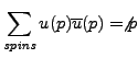 and
and
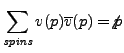 ,
equals
,
equals
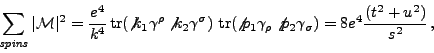
    Vectors k1, k2, p1, p2;
    Symbols s, t, u, e;
    Indices mu, nu, rho, sigma;
    *
    Local   M2 =
    *       electron line
              e^2 * g_(1, k1, rho, k2, sigma) *
    *       photon propagator
              d_(rho,mu) * d_(sigma,nu) / s^2 *
    *       muon spin line
              e^2 * g_(2, p1, mu, p2, nu)
            ;
    Trace4,1;
    Trace4,2;
    Bracket e,s;
    Print;
    .sort

   M2 =
       + s^-2*e^4 * ( 32*k1.p1*k2.p2 + 32*k1.p2*k2.p1 );

    *
    id k1.k2 = s/2;
    id p1.p2 = s/2;
    id k1.p1 = -t/2;
    id k2.p2 = -t/2;
    id k1.p2 = -u/2;
    id k2.p1 = -u/2;
    Bracket e,s;
    Print;
    .end

   M2 =
       + s^-2*e^4 * ( 8*t^2 + 8*u^2 );
The following is an example from high energy physics that illustrates the
efficiency of the trace algorithms that have been implemented in FORM.
We are looking at the reaction
![]() .
This is a 2 to 6 reaction, but it has some features that make it easier
than one might expect.
.
This is a 2 to 6 reaction, but it has some features that make it easier
than one might expect.
    Vectors p1,...,p8,Q,q1,q2;
    Indices m1,m2,m3,n1,n2,n3;
    Symbol emass,tmass,mass4,mass5,mass7,mass8;
    On Statistics;
    Local   F =
    *
    *   The incoming e+ e- pair. momenta p2 and p1
    *
        (g_(1,p2)-emass)*g_(1,m1)
        *(g_(1,p1)+emass)*g_(1,n1)
    *
    *   The tau line. tau- is q1, tau+ is q2.
    *
        *g_(2,p3)*g_(2,m2)*g7_(2)
        *(g_(2,q1)+tmass)*g_(2,m1)
        *(-g_(2,q2)+tmass)*g_(2,m3)*g7_(2)*g_(2,p6)
        *g_(2,n3)*g7_(2)*(-g_(2,q2)+tmass)*g_(2,n1)
        *(g_(2,q1)+tmass)*g_(2,n2)*g7_(2)
    *
    *   The u d-bar pair. p4 is u, p5 is d-bar.
    *
        *(g_(3,p4)+mass4)*g_(3,m2)*g7_(3)
        *(g_(3,p5)-mass5)*g_(3,n2)*g7_(3)
    *
    *   The d u-bar pair. p7 is d, p8 is u-bar.
    *
        *(g_(4,p7)+mass7)*g_(4,m3)*g7_(4)
        *(g_(4,p8)-mass8)*g_(4,n3)*g7_(4)
        ;
    trace4,1;
    trace4,2;
    trace4,3;
    trace4,4;
    contract;
    print +s;
    .end

Time =       0.49 sec    Generated terms =        164
                F        Terms in output =         27
                         Bytes used      =       1354

   F =
       - 524288*p1.p2*p3.p4*p5.p7*p6.p8*q1.q2*tmass^2
       + 524288*p1.p2*p3.p4*p5.q1*p6.p8*p7.q2*tmass^2
       + 524288*p1.p2*p3.p4*p5.q2*p6.p8*p7.q1*tmass^2
       + 262144*p1.p5*p2.p7*p3.p4*p6.p8*q1.q1*q2.q2
       + 524288*p1.p5*p2.p7*p3.p4*p6.p8*q1.q2*tmass^2
       + 262144*p1.p5*p2.p7*p3.p4*p6.p8*tmass^4
       - 524288*p1.p5*p2.q2*p3.p4*p6.p8*p7.q1*tmass^2
       - 524288*p1.p5*p2.q2*p3.p4*p6.p8*p7.q2*q1.q1
       + 262144*p1.p7*p2.p5*p3.p4*p6.p8*q1.q1*q2.q2
       + 524288*p1.p7*p2.p5*p3.p4*p6.p8*q1.q2*tmass^2
       + 262144*p1.p7*p2.p5*p3.p4*p6.p8*tmass^4
       - 524288*p1.p7*p2.q1*p3.p4*p5.q1*p6.p8*q2.q2
       - 524288*p1.p7*p2.q1*p3.p4*p5.q2*p6.p8*tmass^2
       - 524288*p1.q1*p2.p7*p3.p4*p5.q1*p6.p8*q2.q2
       - 524288*p1.q1*p2.p7*p3.p4*p5.q2*p6.p8*tmass^2
       + 524288*p1.q1*p2.q2*p3.p4*p5.p7*p6.p8*tmass^2
       + 1048576*p1.q1*p2.q2*p3.p4*p5.q1*p6.p8*p7.q2
       - 524288*p1.q2*p2.p5*p3.p4*p6.p8*p7.q1*tmass^2
       - 524288*p1.q2*p2.p5*p3.p4*p6.p8*p7.q2*q1.q1
       + 524288*p1.q2*p2.q1*p3.p4*p5.p7*p6.p8*tmass^2
       + 1048576*p1.q2*p2.q1*p3.p4*p5.q1*p6.p8*p7.q2
       + 262144*p3.p4*p5.p7*p6.p8*q1.q1*q2.q2*emass^2
       + 262144*p3.p4*p5.p7*p6.p8*emass^2*tmass^4
       - 524288*p3.p4*p5.q1*p6.p8*p7.q1*q2.q2*emass^2
       + 1048576*p3.p4*p5.q1*p6.p8*p7.q2*q1.q2*emass^2
       + 1048576*p3.p4*p5.q1*p6.p8*p7.q2*emass^2*tmass^2
       - 524288*p3.p4*p5.q2*p6.p8*p7.q2*q1.q1*emass^2
      ;
 and
and
 .
.
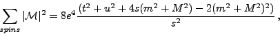
We started the subsection about wildcard parameters with
the simplification
![]() . The implemented
replacement rule worked well for the formula
. The implemented
replacement rule worked well for the formula ![]() , but
look what is the result when applied to
, but
look what is the result when applied to ![]() .
.
    Symbol a,x,y;
    CFunction sqrt;
    Local F = 2 * sqrt(a);
    id x? * sqrt(y?) = sqrt(x^2*y);
    Print;
    .end

   F =
      2*sqrt(a);
The coefficient is not recognized in the wildcarding.
In FORM, you cannot write an identification like 2*sqrt(y?).
The best workaround is to put the coefficient inside a dummy function
via the PolyFun option to a FORM directive.
Then you can write the replacement which involves coefficients. In our
example it could look like
    Symbol a,x,y;
    CFunctions sqrt,dummy;
    Local F = 2 * sqrt(a);
    Print;
    .sort (PolyFun = dummy);

   F =
      sqrt(a)*dummy(2);

    id dummy(x?) * sqrt(y?) = sqrt(x^2*y);
    Print;
    .end

   F =
      sqrt(4*a);
The semicolon at the end of the PolyFun option is
obligatory. This statement is an example of a module option statement.
There can be more than one module option statement.
The module option statement(s) are the last statement(s) before the
FORM directives at the end of the module.
They are local settings that overwrite more general settings.
They hold only for the current module.
Another working style is to use a PolyFun declaration.
Like any other declaration it will remain valid during the session
and does not have to be put in all .sort instructions.
The declaration PolyFun; switches the PolyFun option off.
So, we can also use the following FORM program:
    Symbol a,x,y;
    CFunctions sqrt,dummy;
    Polyfun dummy;
    Local F = 2 * sqrt(a);
    Print;
    .sort
    Polyfun;
    id dummy(x?) * sqrt(y?) = sqrt(x^2*y);
    Print;
    .end
Another way of getting hold of the coefficients is by use of the
collect statement. With this statement you can put data
which are between brackets (either by the Bracket or AntiBracket
statement) inside a regular function. Our example would look like
    Symbol a,x,y;
    CFunctions sqrt,dummy;
    Local F = 2 * sqrt(a);
    AntiBracket a;
    Print;
    .sort

   F =
       + sqrt(a) * ( 2 );

    collect dummy;
    Print;
    .sort

   F =
      sqrt(a)*dummy(2);


    id dummy(x?) * sqrt(y?) = sqrt(x^2*y);
    Print;
    .end

   F =
      sqrt(4*a);
Another type of pattern matching which is currently not allowed in FORM is f(x?+y?), and variations thereof. For example,
additivity of a function f cannot be specified as follows:
    Symbols x,y,z;
    CFunction f;
    Local expr = f( x + y + z );
    id f( x? + y? + z? ) = f(x) + f(y) + f(z);
    Print;
    .end

   expr =
      f(x + y + z);
The reason for not allowing this kind of wildcarding in function arguments
is efficiency: the pattern f(x1?+x2?+...+xn?) has in general
However, the above problem of additivity of a function can be implemented by the following trick. In fact, we implement more: linearity of a function.
    Vectors x,y,z;
    Index i;
    CFunction f;
    Local expr = f( 2*x + y + z );
    id f(i?) = f(i);
    Print;
    .end

   expr =
      2*f(x) + f(y) + f(z);
The explanation is as follows: the wildcard in the function is an index.
If FORM gets a vectorlike argument in the function, it assumes that it
is there because of contraction of indices. In other words, it assumes
that the function is linear in this argument.
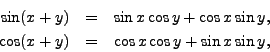
FORM provides the usual facilities of procedural programming languages: control flow statements such as repetition with ``do''- and ``while''-loops and choice control structures of type ``if-then-else'' and ``switch'' are present, and procedures can be defined and called as one pleases. There is however an important difference with many languages: FORM consists of two parts, viz., the preprocessor and the compiler. At both levels, tools of procedural programming are provided. In this section we shall describe the functionality of the preprocessor. In the second section, the programming facilities at compiler level will be discussed.
The preprocessor reads from the input stream and prepares input for the compiler. The preprocessor prepares program blocks, also called modules, which are translated by the compiler, and immediately executed. As such, you can consider the preprocessor as an autonomous unit that facilitates the efficient and easy writing of FORM programs. A command for the preprocessor is called a preprocessor instruction. It always starts with the sharp symbol (#), it does not have to end with a semicolon, and it is executed when it is encountered in the input stream. Preprocessor instructions are there to make programming in FORM easier. For example, the preprocessor has its own structures for control flow and it allows you to write procedures. To make preparation of code for the compiler easier, the preprocessor is equipped with variables that can be defined or redefined by the user or by other preprocessor actions. The preprocessor variables can be recognized by the quotes that are around them when they are referred to. In this section we shall concentrate on the control flow preprocessor instructions and the preprocessor variables; the preprocessor instructions that have to do with I/O will be discussed in a later chapter.
The conditional statement in the preprocessor provides a way to include code selectively. Formally, it has the following syntax.
#if condition
[#else
]
#endif
#endif instruction marks the end of the choice.
The condition is evaluated: if it is true, i.e., if it has a non-zero
value,
#endif instruction.
If condition is false, i.e., if it is zero, and if there is
an else part,
#if `i'
#endif
#if `i' != 0
#endif
`i' has a value that can be interpreted as a number. If there is just a
string, and not a number, the condition is false.
A composite condition is composed of variables and numbers via relational operators (less than, equal to, etc.) and logical operators (and, or). The operator are tabulated below. Relational operators are in FORM mostly the same as in the C programming language and are either numerical comparisons or string comparisons with respect to the lexicographic ordering of strings. The same holds for logical operators, with the exception that the negation (!) does not exist in FORM.
| Operator | Meaning |
| = or == | equal to |
| != | not equal to |
| greater than | |
| less than | |
| greater than or equal to | |
| less than or equal to | |
| && | and |
| or |
A typical #if statement is
#if {`i'%2} == 0
  1
#else
  -1
#endif
where `i' is a preprocessor variable, which is defined elsewhere in the
FORM program, and where we have used the percentage symbol
% for modular arithmetic
(if part are required for this behavior.
Otherwise, the preprocessor does not carry out the remainder calculation and
it will compare two very different strings, viz., i%2 and 0.
This behavior will become more clear after preprocessor variables and
their calculus have been discussed.
Nested #if statements are allowed, and FORM provides the shortcut
#elseif.
#if `x' < 0
  -1
#else
  #if `x' = 0
    0
  #else
    1
  #endif
#endif
is equivalent to#if `x' < 0 -1 #elseif `x' = 0 0 #else 1 #endif
The following sequence of #if, #elseif, #else, and
#endif instructions is the most general way of writing a multi-way
decision.
#if
#elseif
#elseif
#elseif
#else
#endif
#endif instruction.
The last #else part handles the ``none of the above'' or default case
where none of the other conditions is satisfied. If there is no explicit
reading required for the default, the #else part can be omitted, or
it can be used for error checking an ``impossible'' condition.
The #switch instruction, together with #break,
#default, and #endswitch, provides a multi-way decision,
which tests whether a string matches one of a number of constant string
values, and which branches accordingly.
In other words, these instructions allow the user to conveniently make
code for a number of cases that are distinguished by the string value of a
preprocessor variable.
#switch
#case
#break
#case
#break
#case
#break
#case
#break
[#default
#break]
#endswitch
#switch
instruction and, if found, starts at that case.
The case labeled #default is read if none of the other cases are
satisfied.
The #default case can be omitted: then, if none of the cases match,
reading just continues after the #endswitch instruction, i.e., no action
at all takes place.
The #break instruction causes an immediate exit from the switch.
It prevents that after the code of one case is read, processing
falls through to the next case.
Let us have the conditional statements of the previous sections in an executable FORM program.
    #define two "2"
    #define three "3"
    #define four "4"
    #define quatro "4"
    Symbols x2,...,x5;
    Local F`two' =
    #if {`two'%2} == 0
       1
    #else
      -1
    #endif
    ;
    Local F`three' =
    #if {`three'%2} == 0
       1
    #else
      -1
    #endif
    ;
    Local F`four' =
    #switch {`four'/2}
    #case {`quatro'/2}
      + x2
    #case `three'
      + x3
    #break
    #case 2
      + x4
    #default
      + x5
    #endswitch
    ;
    Print;
    .end

   F2 =
      1;

   F3 =
       - 1;

   F4 =
      x2 + x3;
With the #define instruction you can give a
string value to a preprocessor variable. Of course, the string values
in our example have a numerical interpretation, and the preprocessor
knows this. It concatenates regular string characters and preprocessor
variables: the names F2, F3, and F4 of the local
expressions in the above session are constructed in this way. Furthermore,
you can do arithmetic operations with preprocessor variables that have a
numerical interpretation: in our example, we compute the remainder and
quotient of division by two.
Be warned that the preprocessor does not always interpret string values numerically or in the same way as you would do. For example, rational numbers are rounded to integers (in the direction to zero) before any further processing, in case curly brackets are present. The following FORM session illustrates this.
    #define minustwothird "-2/3"
    Local expr1a = `minustwothird';
    Local expr1b =
    #if `minustwothird' > -3/2
       1
    #elseif `minustwothird' == 0
       0
    #else
      -1
    #endif
    ;
    Local expr1c =
    #if {`minustwothird'} > -3/2
       1
    #elseif {`minustwothird'} == 0
       0
    #else
      -1
    #endif
    ;
    Local expr1d = {`minustwothird'};
    Print;
    .end

   expr1a =
       - 2/3;

   expr1b =
       - 1;

   expr1c =
      1;

   expr1d = 0;
Again, the curly brackets get the integer calculator of the preprocessor
activated while reading the input stream.
In general, three types of repetitions can be distinguished
![]() Counted Do-Loop
Counted Do-Loop
The preprocessor provides two types of unconditional do-loops. The first one is similar to the one found in most programming languages, and is referred to as a counted do-loop.
#docounter=start,finish [,stepsize ]
statseq
#enddo
#enddo instruction. statseq represents
any valid FORM expression, statement, or sequence of statements
separated by semicolons, which are read at each step in the repetition.
The stepsize is optional: if omitted, the default value 1
will be assumed. You cannot alter the finish and stepsize from
within the loop; it is however allowed to redefine the preprocessor
variable counter. Furthermore, the preprocessor variable used
for counting has no value or no meaning outside the loop.
In the following four examples, we compute the sum of the first ten natural
numbers with the preprocessor. The first session uses a simple
#do loop to compose an expression that is by definition equal to the
requested sum.
    Local S =
    #do i = 1, 10
       + `i'
    #enddo
    ;
    Print;
    .end

   S =
      55;
A preprocessor variable can be used to make the program more general.
    #define MAX "10"
    Local S =
    #do i = 1, `MAX'
       + `i'
    #enddo
    ;
    Print;
    .end

   S =
      55;
The above two sessions were just there for explaining the simple counted
do-loop. In a real FORM program, it is of course easier to use the
following code, which is also more readable.
    #define MAX "10"
    Local S = 1 + ... + `MAX';
    Print;
    .end

   S =
      55;
Counted do-loops can be nested.
    Local S =
    #do i = 1, 5
       #do j = 0, 1
          + 2*`i' - `j'
       #enddo
    #enddo
    ;
    Print;
    .end

   S =
      55;
In the above three do-loop programs we have used the #do to compose
a local expression. This is why we always have a semicolon after the
#enddo instruction on a separate line in the above programs.
Of course the loop control structure can also be used with ``complete''
FORM statements.
    Local S0 = 0;
    #do i = 1, 10
        Local S`i' = S{`i'-1} + `i';
    #enddo
    Print S10;
    .end

   S10 =
      55;
The start, finish, and stepsize of a counted do-loop do not need to be
integers:
rationals will also do because the preprocessor's arithmetic will always
give an integer result. The following rather weird example illustrates that
FORM does its best to make sense of the instructions.
    AutoDeclare Symbol x;
    Local S =
    #do i = -2, 9/2, 3/2
       + x`i'
    #enddo
    ;
    Print;
    .end

   S =
       - 3 + 2*x + x0 + x1 + x2 + x3 + x4;
First of all the finish and stepsize of the loop are calculated via integer
division as 4 and 1, respectively. The concatenation of strings ``x-1'' and
``x-2'' for i = -1 and i = -2 lead to the summands 2*x-3
in the end result.
![]() Listed Do-Loop
Listed Do-Loop
The second variation on the #do loop is the listed
do-loop.
#doname= {sequence}
statseq
#enddo
    Indices i,j,k;
    Function T;
    Local expr =
    #do p = {1,i|2\,i|j,(k,k)}

      + T(`p')
    #enddo
    ;
    Print;
    .end

   expr =
      T(k + T(k)) + T(i) + T(j) + T(1) + T(2,i);
We ``escape'' a comma in 2\,i so that it is read as one parameter with
string value "2,i" and so that it gives the last term in the above
expression.
The first term in the output is a bit strange: it shows that FORM indeed
picks the terms between the round brackets in one step of the loop and
processes them recursively, one by one, from left to right.
![]() Realistic Examples of Unconditional Do-Loops
Realistic Examples of Unconditional Do-Loops
We end this subsection about unconditional repetition with three,
more realistic examples of unconditional #do loops.
In the first example we are going to take the series expansion of
![]() about
about ![]() up to 50 terms and substitute in it the series
expansion of
up to 50 terms and substitute in it the series
expansion of ![]() about
about ![]() . The expansions we need are:
. The expansions we need are:
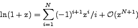
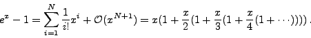
    * check that exp(ln(1+x))-1 = x up to order 50 in series expansions
    #define N "50"
    On Statistics;
    Symbol i, x(:`N'), y(:`N');
    *   define ln(1+x)
    Local X =  - sum_(i, 1, `N', sign_(i)/i*x^i);
    *   tag x by y
    id  x = x*y;
    *   so that we can use the telescope formula of exp(x)-1.
    *   in this example, the expansion will be slow.
    #do i=2,'N'+1
        id  y = 1 + x*y/`i';
    #enddo
    * print the result
    Print;
    .end

Time =    1068.25 sec    Generated terms =    1295970
                X        Terms in output =          1
                         Bytes used      =         18

   X =
      x;
The program gives the expected answer .sort instruction inside the loop. Then, only about 15000 terms are
generated during the computation.
    * check that exp(ln(1+x))-1 = x up to order 50 in series expansions
    #define N "50"
    On Statistics;
    Symbol i, x(:`N'), y(:`N');
    *   define series expansion of ln(1+x)
    Local X =  - sum_(i, 1, `N', sign_(i)/i*x^i);
    *   tag x by y
    id  x = x*y;
    *   so that we can use the telescope formula of exp(x)-1.
    *   in this example, sorting takes place at each step of the expansion.
    #do i=2,'N'+1
        id  y = 1 + x*y/`i';
        .sort: step `i';

Time =       1.12 sec    Generated terms =        675
                X        Terms in output =        675
                 step 2  Bytes used      =       9638
    #enddo

Time =       3.79 sec    Generated terms =       4247
                X        Terms in output =        433
                 step 3  Bytes used      =       7182

Time =       4.97 sec    Generated terms =       2206
                X        Terms in output =        348
                 step 4  Bytes used      =       7030
  .
  .
  .

Time =       8.42 sec    Generated terms =          6
                X        Terms in output =          3
                step 50  Bytes used      =        158

Time =       8.43 sec    Generated terms =          3
                X        Terms in output =          1
                step 51  Bytes used      =         18
    * print the result
    Print;
    .end

Time =       8.43 sec    Generated terms =          1
                X        Terms in output =          1
                         Bytes used      =         18

   X =
      x;
We have added a commentary to the .sort
instruction so that the statistics shows which step of the do-loop is involved.
The commentary to the module instruction is initiated by a
colon, it is terminated by a semicolon, and the characters in between form
the message printed.
The second example is about simplifying an expression in a
6-dimensional Clifford algebra generated by elements
![]() with relations
with relations
#do loop for this purpose.
    #define DIM "6";
    Symbols i;
    Functions e;
    Local  expr = sum_(i, 1, `DIM', e(i)) ^ 3;
    repeat;
      #do i = 1, `DIM'
         #do j = `i'+1, `DIM'
             id e(`j') * e(`i') = -e(`i') * e(`j');
         #enddo
         id e(`i') * e(`i') = 1;
      #enddo
    endrepeat;
    Print;
    .end

   expr =
      6*e(1) + 6*e(2) + 6*e(3) + 6*e(4) + 6*e(5) + 6*e(6);
The third example is about computing Fibonacci numbers ![]() ,
which are recursively defined by
,
which are recursively defined by
    #define MAX "7"
    Local F1 = 1;
    Local F2 = 1;
    #do n = 3, `MAX'
       .sort
       Drop F{`n'-2};
       Skip F{`n'-1};
       Local F`n' = F{`n'-1} + F{`n'-2};
       Print;
    #enddo

   F3 =
      2;


   F4 =
      3;


   F5 =
      5;


   F6 =
      8;

    .end

   F7 =
      13;
There are more reasons for showing this example. It makes once more clear that
curly brackets, instead of round brackets, are used to set precedence in the
preprocessor. But we also want to point out the Drop and Skip
instruction. When the Drop statement is used,
the expression can be used in the current module, but after the next
.sort or .store instruction the expression does not exist
anymore.
The Skip instruction inactivates the expression only for the range
of the current module. The skipped expression may be used in the right hand
side of an identification, but no operation is performed on the expression
in the current module. In our example, this means that we forget
about Fibonacci numbers when they are not needed anymore in the recursive
computation. Furthermore, when it comes to printing of results, we
forget about the Fibonacci number computed in the previous step; we only
show the result of the newly computed number. The printing is inside the
loop; therefore the .end instruction appears in the above output
much later than in the source file, where it is just after the #enddo
instruction.
The following example, in which the Fibonacci number ![]() is computed,
shows how a conditional repetition like a post-checked do-loop can be
constructed. Other conditional repetitions can be treated similarly.
is computed,
shows how a conditional repetition like a post-checked do-loop can be
constructed. Other conditional repetitions can be treated similarly.
    Symbol x;
    Local F19 = x^18;
    #do i = 1, 1
       id x^2 = x+1;
       if (count(x,1)>1) redefine i "0";
       .sort
    #enddo
    id x = 1;
    Print;
    .end

   F19 =
      4181;
As long as there exist powers of count function is for power counting --
we reset the preprocessor variable to the value 0 inside the loop. In effect,
the do-loop becomes a post-checked do-loop.
A few remarks about the above FORM code are still necessary. The condition,
which determines whether the loop should be terminated or not, is checked
during program execution, via a regular if statement.
The redefinition of the loop variable i is not carried
out by the preprocessor instruction #redefine, but instead
by a regular command called redefine, because
it is part of a choice control structure at compiler level and not at
preprocessor level.
This command should be before the last .sort inside the loop,
because the #do instruction is part of the preprocessor. This implies
that the value of the loop variable i is considered before the module
is executed. This means that if the redefine command would be after
the last .sort inside the loop, two things would go wrong: First,
the loop would be terminated before the redefine command would ever
make a chance of being executed. Secondly, the statement would be compiled
in the expectation that there exists a variable i, but then the loop
would be terminated.
Afterwards, when the statement is being executed, the redefine statement
would refer to a variable that does not exist anymore.
The above construction can also be used to simulate a kind of
multi-module repeat; as we shall see in the next section, the
repeat loop may only contain statements from within a single module.
The code will look as follows:
#do i = 1, 1
some statements
if ( match(pattern) ) redefine i "0";
.sort
#enddo
As long as there are terms with the pattern -- the match
function will select them -- the statements will be
repeated. Note that if there are more expressions, they will all be repeated,
even those expressions that do not contain the pattern any longer.
The above code emulates a do-until loop that can contain one or more
.sort instructions. In subsection 3.1.5 we shall use
this kind of control structure in processing word problems in
Coxeter groups.
In order to help in the preparation of code for the compiler, the preprocessor is equipped with variables that can be defined or redefined by the user or by other preprocessor actions. We have already seen examples of preprocessor variables in the choice and repetition examples of the previous subsections. Preprocessor variables have regular names that are composed of strings of alphanumeric characters of which the first must be alphabetic. Recall that FORM is case-sensitive with respect to variables. In the table below we list all preprocessor instructions that deal with definition and removal of preprocessor variable.
| Instruction | Meaning |
#define var "string" |
initialize the preprocessor variable var with the string value |
#redefine var "string" |
(re)set the preprocessor variable var to the string value |
#undefine var |
remove the preprocessor variable var |
The preprocessor variables can be recognized in a FORM program and be
distinguished from regular variables by the quotes that are around them
when they are referred to. This convention makes it possible to concatenate
regular strings of character and preprocessor variables to form larger
strings of characters. The following example, which involves
four preprocessor variables, viz., `i', `j', `MAX', and
`max', illustrates the concatenation of strings.
    #define MAX "2"
    #define max "2"
    AutoDeclare Symbol x;
    #do i = 1, `MAX'
       #do j = 1, `max'
          Local F`i'`j' = x^`i'`j';
       #enddo
    #enddo
    Print;
    .end

   F11 =
      x^11;

   F12 =
      x^12;

   F21 =
      x^21;

   F22 =
      x^22;
The left and right quotes can be nested. Hence `max`i''
will result in the preprocessor variable i to be substituted first. If
it happens to be the string "1", the result after the first substitution
is max1 and then FORM first looks up its string value.
This explains the following session.
    #define max1 "2"
    #define max2 "3"
    AutoDeclare Symbol x;
    #do i = 1, 2
       #do j = 1, `max`i''
          Local F`i'`j' = x^`i'`j';
       #enddo
    #enddo
    Print;
    .end

   F11 =
      x^11;

   F12 =
      x^12;

   F21 =
      x^21;

   F22 =
      x^22;

   F23 =
      x^23;
When the preprocessor encounters a left curly bracket it will read till the matching right curly bracket and test whether the characters, after substitution of the preprocessor variables, can be interpreted numerically. If so, the preprocessor calculator will compute the numeric result and the original string is replaced by a textual representation of the number computed. If no numerical interpretation of an expression between curly brackets is possible, the whole string, including the curly brackets, will be passed on to the later stages of the FORM program. An example is the FORM program of the previous section, in which Fibonacci numbers were computed: the statement
Local F`n' = F{`n'-1} + F{`n'-2};
Local F6 = F5 + F4;
`n' has the value 6.
A valid numerical expression can contain digits and the characters +,
-, *, /, ^, %, !, &,
![]() ,
, (, ), {, and }.
Very important is that the comma , is not a legal
character for the preprocessor calculator. This explains the difference
between
if f(x?!{0}) = 1/x;
which the preprocessor changes into the syntacticly incorrect statement
if f(x?!0) = 1/x;and the statement
if f(x?!{0,0}) = 1/x;
which the preprocessor leaves untouched, because of the presence of the comma,
so that the identify statement is carried out for nonzero x.
Parentheses ( ) and curly brackets { } are used for setting
priority rules in preprocessor calculations. The other characters listed
above occur in arithmetic operators. All arithmetic is done over integers
in a finite range: from
| Operator | Meaning |
+ |
addition |
- |
subtraction |
* |
multiplication |
/ |
division |
^ |
exponentiation |
% |
remainder after division |
! |
factorial |
& |
bitwise AND (as in C) |
^% |
a postfix
|
^/ |
a postfix integer square root |
One of the most important features of the preprocessor is the use of procedures. A FORM procedure has the following syntax
#procedure name [ ( parameterseq ) ]
statements
#endprocedure
#call instruction, which has the following
syntax
#call name [ ( argumentseq ) ]
where the argumentseq is a sequence of FORM expressions
separated by commas or vertical bars (as in the listed do-loop).
If the definition of a procedure has no parameters, the procedure call
should not contain arguments either.
Let us look at an example: the Fibonacci numbers again.
    #procedure fibonacci(F,n)
    *
    * Procedure to compute Fibonacci numbers
    * Input: F: the function that represents the number
    * It should have one argument, viz. n, which is
    * for internal use and must be declared as a symbol
    * before the procedure call.
    *
      repeat;
        id `F'(1) = 1;
        id `F'(2) = 1;
        id `F'(`n'?) = `F'(`n'-1) + `F'(`n'-2);
      endrepeat;
    #endprocedure

    Symbol n;
    CFunction F;
    On Statistics;
    Local F19 = F(19);
    #call fibonacci(F,n)
    Print;
    .end

Time =       6.71 sec    Generated terms =       4181
              F19        Terms in output =          1
                         Bytes used      =         10

   F19 =
      4181;
Although the procedure looks like a subroutine, it works in fact more like a
macro. When the procedure is called, the preprocessor checks whether the
procedure is defined, and if so, whether the number of arguments matches the
number of parameters in the procedure definition. When everything seems to
be okay, the preprocessor substitutes the program block. In our example, the
program block consists of a repetition of identifications that compute the
requested Fibonacci number by downward recursion
(as in Section 2.3.2).
The very deep recursion in the above procedure is rather costly.
One way to solve this problem is to tabulate the ten
lowest Fibonacci numbers.
Then the reduction stops when a table element is reached. This brings
us to the creation of tables in FORM. A table is a special function in
FORM: it is a kind of array filled with data. A table must be declared
first with the Table statement and it must be filled before any
executable statement. It declares the table automatically as a commuting
function. This could have been done more explicitly via the CTable
instruction. A noncommuting table is declared with the NTable
instruction.
The array can be multidimensional, be of special type such as ``sparse'',
and have wildcards as formal parameters. The creation of
a table of Fibonacci numbers and its use goes as follows.
    #define MAXTAB "10"
    Table Ftbl(1:`MAXTAB');
    Fill Ftbl(1) = 1;
    Fill Ftbl(2) = 1;
    #do i = 3, `MAXTAB'
       Fill Ftbl(`i') = Ftbl({`i'-1}) + Ftbl({`i'-2});
    #enddo

    #procedure fibonacci(F,n)
    *
    * Procedure to compute Fibonacci numbers
    * Input: F: the function that represents the number
    * It should have one argument, viz. n, which is
    * for internal use and must be declared as a symbol
    * before the procedure call.
    *
      id `F'(?x) = Ftbl(?x);    * replace F by Ftbl
      repeat;
        id Ftbl(`n'?) = Ftbl(`n'-1) + Ftbl(`n'-2);
      endrepeat;
    #endprocedure

    Symbol n;
    CFunction F;
    On Statistics;
    Local F19 = F(19);
    #call fibonacci(F,n)
    Print;
    .end

Time =       0.89 sec    Generated terms =       4181
              F19        Terms in output =          1
                         Bytes used      =         10

   F19 =
      4181;
The curly brackets in the statement
Fill Ftbl(`i') = Ftbl({`i'-1}) + Ftbl({`i'-2});
are essential for efficient use of the table. Of course, the first part of
the above program could have been used on its own
to compute the nineteenth Fibonacci number.
    #define MAXTAB "19"
    Table Ftbl(1:`MAXTAB');
    Fill Ftbl(1) = 1;
    Fill Ftbl(2) = 1;
    #do i = 3, `MAXTAB'
       Fill Ftbl(`i') = Ftbl({`i'-1}) + Ftbl({`i'-2});
    #enddo
    On Statistics;
    Local F19 = Ftbl(19);
    Print;
    .end

Time =       0.61 sec    Generated terms =       4181
              F19        Terms in output =          1
                         Bytes used      =         10

   F19 =
      4181;
However, this is still not the most efficient FORM program to compute the
Fibonacci number. Nevertheless, it is a clear and easy implementation.
The version below, which we have explained before, is the fastest
(CPU-time 6 times faster) and the least memory consuming, but it is
a little bit more complicated.
    #define MAX "19"
    On Statistics;
    Local F1 = 1;
    Local F2 = 1;
    #do n = 3, `MAX'
       .sort
       Drop F{`n'-2};
       Skip F{`n'-1};
       Local F`n' = F{`n'-1} + F{`n'-2};
    #enddo
    Print;
    .end
The .sort, Drop, and Skip are essential for the
efficiency. They make that not 4181 terms are generated but only
As a second example of the use of procedures in FORM, we rewrite our example of differentiation of trigonometric functions from Section 2.5.3.
    #procedure diff(x,dx)
      id g?commuting?noncommuting(`x') = g(`x');
      Multiply left `dx';
      repeat;
        id `dx'*g?noncommuting[n](`x') = derivative[n](`x') + g(`x')*`dx';
        id [-sin](`x') = - [sin](`x');
        id [1/cos^2](`x') = 1/[cos](`x') * 1/[cos](`x');
      endrepeat;
      id `dx' = 0;
      id f?noncommuting?commuting(`x') = f(`x');
      id 1/f?noncommuting?commuting(`x') = 1/f(`x');
    #endprocedure
    *
    * The following statements could be put in a standard include file
    *
    Symbols x,n;
    CFunctions sin,cos,tan,g;
    Functions [sin], [cos], [tan], [-sin], [1/cos^2], f, dx;
    Set commuting: sin, cos, tan;
    Set noncommuting: [sin], [cos], [tan];
    Set derivative: [cos], [-sin], [1/cos^2];
    FunPowers allfunpowers;
    *
    * And the rest of the program is as follows
    *
    Local expr = sin(x)*tan(x) + cos(x);
    #call diff(x,dx)
    Print;
    .end

   expr =
       - sin(x) + cos(x)*tan(x) + 1/(cos(x))^2*sin(x);
The comments are even more important here as they give a clue to how
to work more easily with FORM. In our example, we can put the differentiation
procedure in a file called diff.prc, without the left and right quotes
around the parameters. The accompanying declarations can be stored
in a file called diff.h (the declarations of x, and dx
are kept outside). The two files look as follows.
    #procedure diff(x,dx)
      id g?commuting?noncommuting(x) = g(x);
      Multiply left dx;
      repeat;
        id dx*g?noncommuting[n](x) = derivative[n](x) + g(x)*dx;
        id [-sin](x) = - [sin](x);
        id [1/cos^2](x) = 1/[cos](x) * 1/[cos](x);
      endrepeat;
      id dx = 0;
      id f?noncommuting?commuting(x) = f(x);
      id 1/f?noncommuting?commuting(x) = 1/f(x);
    #endprocedure
    #-
    Symbols n;
    CFunctions sin,cos,tan,g;
    Functions [sin], [cos], [tan], [-sin], [1/cos^2], f, dx;
    Set commuting: sin, cos, tan;
    Set noncommuting: [sin], [cos], [tan];
    Set derivative: [cos], [-sin], [1/cos^2];
    FunPowers allfunpowers;
    #+
Now, the program can just look like
    #include diff.h
    Symbol x;
    Function dx;
    Local expr = sin(x)*tan(x) + cos(x);
    #call diff(x,dx)
    Print;
    .end
How does it run under FORM? When the preprocessor encounters the
#include diff.h, it inserts the contents of
the file into the input.
The #- instruction means that the listing of the
input, when running the program, will be turned off until further notice.
With the #+ instruction, logging of input is resumed again. We added
these instructions in the file diff.h because normally it is
unnecessary to see the declarations needed for the procedure definition.
When the preprocessor encounters the procedure call, it will first look
whether there is a definition in the program given. If not, it will
look for the definition in a file whose name is the name of the procedure
extended with .prc. This file is searched for in the current directory
or in the directories listed in the environment variable FORMPATH or
indicated by the -p option in the command that starts the system.
The proof of the pudding is in the eating: let
us run the FORM program.
    #include diff.h
    #-
    Symbol x;
    Function dx;
    Local expr = sin(x)*tan(x) + cos(x);
    #call diff(x,dx)
    Print;
    .end

   expr =
       - sin(x) + cos(x)*tan(x) + 1/(cos(x))^2*sin(x);
We end with a few remarks about procedures in FORM.
nargs_
function.
What we have learned so far in this chapter can be applied in a realistic FORM application: processing word problems in Coxeter groups.
Following [du Cloux 99], let us first give a brief introduction to the
topic. A Coxeter system is a pair ![]() consisting of a group
consisting of a group
![]() and a set of generators
and a set of generators ![]() , subject only to relations of
the form
, subject only to relations of
the form
For example, the symmetric group ![]() of all permutations of a
sequence of
of all permutations of a
sequence of ![]() objects, with the following
objects, with the following ![]() adjacent transpositions
as generators
adjacent transpositions
as generators ![]() ,
,
![]() forms a
Coxeter group with Coxeter graph
forms a
Coxeter group with Coxeter graph
For a Coxeter system ![]() , the generators
, the generators ![]() have order 2 in
have order 2 in ![]() .
Hence, each element
.
Hence, each element ![]() in
in ![]() can be written in the form
can be written in the form
![]() for some
for some ![]() (not necessarily distinct) in
(not necessarily distinct) in ![]() . If
. If
![]() is as small as possible, we call it the length of
is as small as possible, we call it the length of ![]() ,
written
,
written ![]() , and call any expression of
, and call any expression of ![]() as a product of
as a product of ![]() elements of
elements of ![]() a reduced expression.
The Poincaré series of
a reduced expression.
The Poincaré series of ![]() is the formal power series
is the formal power series ![]() in
indeterminate
in
indeterminate ![]() defined by
defined by
 .
.
Let ![]() be an arbitrary subset of
be an arbitrary subset of ![]() and denote by
and denote by ![]() the subgroup
generated by
the subgroup
generated by ![]() . Furthermore, define the set
. Furthermore, define the set
![]() . Then, each left coset
. Then, each left coset ![]() contains a unique element
contains a unique element ![]() of minimal length,
of minimal length,
![]() for all
for all ![]() ,
and
,
and
![]() . It follows that each
. It follows that each ![]() can be uniquely written as
product
can be uniquely written as
product ![]() with
with ![]() and
and ![]() such that
such that
![]() .
.
We choose once and for all an increasing sequence of subsets
![]() , with
, with ![]() for
for
![]() and define
and define ![]() as the subgroup of
as the subgroup of ![]() generated by
generated by ![]() .
We also set
.
We also set
![]() , for
, for ![]() . Then, the canonical
multiplication map
. Then, the canonical
multiplication map
![]() from
from
![]() to
to ![]() is bijective.
The decomposition
is bijective.
The decomposition
![]() of a group element
of a group element ![]() given by the
previous bijection is called the special decomposition of
given by the
previous bijection is called the special decomposition of ![]() .
We also have chosen now a linear ordering on
.
We also have chosen now a linear ordering on ![]() : the first element is
the unique element of
: the first element is
the unique element of ![]() , the second one is the unique element of
, the second one is the unique element of ![]() not in
not in ![]() , and so on. This allows us to define a well-ordering on the free
monoid
, and so on. This allows us to define a well-ordering on the free
monoid ![]() on the set
on the set ![]() by ordering words first by length, then
lexicographically from the left in each given length. We call this the
ShortLex ordering.
by ordering words first by length, then
lexicographically from the left in each given length. We call this the
ShortLex ordering.
For each ![]() we denote by
we denote by ![]() the unique smallest reduced
expression for
the unique smallest reduced
expression for ![]() in the ShortLex ordering.
in the ShortLex ordering. ![]() is called the
normal form of
is called the
normal form of ![]() with respect to the ShortLex
ordering. In principal, the normal form of
with respect to the ShortLex
ordering. In principal, the normal form of ![]() can be recursively found as
follows:
The normal form of the identity element is the empty string. Let
can be recursively found as
follows:
The normal form of the identity element is the empty string. Let ![]() ,
then
,
then
![]() , where
, where ![]() is the smallest
generator
is the smallest
generator ![]() such that
such that ![]() . We say here ``in principle''
because we have no effective way described yet to determine which
. We say here ``in principle''
because we have no effective way described yet to determine which ![]() satisfy the length condition
satisfy the length condition ![]() .
.
From
![]() one can recursively read off the special
decomposition
one can recursively read off the special
decomposition
![]() in the following way.
Define
in the following way.
Define ![]() to be the smallest integer
to be the smallest integer ![]() such that
such that ![]() ,
,
![]() if there is no such integer. Then
if there is no such integer. Then
![]() ,
,
![]() if
if ![]() , and
, and
![]() .
Roughly stated, the term
.
Roughly stated, the term ![]() can be read off from
can be read off from ![]() as the last
``slice'' taken from the first appearance of the generator
as the last
``slice'' taken from the first appearance of the generator ![]() (empty
if there is no such appearance).
Continue with
(empty
if there is no such appearance).
Continue with
![]() in a similar way to compute
in a similar way to compute
![]() , and so on.
, and so on.
A rewrite system in the free monoid ![]() on
the set of generators
on
the set of generators ![]() is a set of ordered pairs
is a set of ordered pairs
![]() ,
with
,
with ![]() in the ShortLex ordering for each
in the ShortLex ordering for each
![]() ;
we shall write
;
we shall write
![]() instead of
instead of ![]() . If a word
. If a word ![]() contains the left-hand side of a rule
contains the left-hand side of a rule
![]() as an interval,
i.e., if
as an interval,
i.e., if ![]() for some
for some ![]() , we say that the rule
, we say that the rule
![]() applies to
applies to ![]() and that
and that ![]() is the reduction of
is the reduction of ![]() corresponding to
corresponding to
![]() . If none of the rules in
. If none of the rules in ![]() applies to
applies to ![]() , we
say that
, we
say that ![]() is
is ![]() -reduced. Because reductions are
strictly decreasing in the ShortLex ordering, one can obtain from a given word
an
-reduced. Because reductions are
strictly decreasing in the ShortLex ordering, one can obtain from a given word
an ![]() -reduced word in a finite number of steps, i.e.,
all sequences of rewrites terminate.
However, several distinct
-reduced word in a finite number of steps, i.e.,
all sequences of rewrites terminate.
However, several distinct ![]() -reduced words might be obtained from
a given word. A rewrite system is said to be confluent or complete
if each word possesses a unique
-reduced words might be obtained from
a given word. A rewrite system is said to be confluent or complete
if each word possesses a unique ![]() -reduction, which is also
referred to as the
-reduction, which is also
referred to as the ![]() -normal form of the word.
The rewrite system is reduced if the following conditions hold:
-normal form of the word.
The rewrite system is reduced if the following conditions hold:
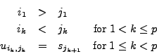
Type
![]()
Completion gives the following ![]() rules:
rules:
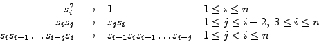
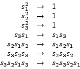
Type
![]()
Completion gives the following ![]() rules:
rules:
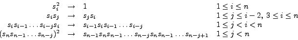
The FORM session below shows the result of computing all elements
of the group ![]() via the above rewrite system for the Coxeter group of
type
via the above rewrite system for the Coxeter group of
type ![]() and the result of computing the Poincaré polynomial.
The calculation is set up in such a way that it works for any Coxeter
group of type
and the result of computing the Poincaré polynomial.
The calculation is set up in such a way that it works for any Coxeter
group of type ![]() . Further explanation follows immediately after the
sample session.
. Further explanation follows immediately after the
sample session.
    #define n "3"
    * define a procedure to generate reduction rules
    #procedure reduce()
        id s?^2 = 1;
        #do i = 3,`n'
          #do j = 1,{`i'-2}
            id s`i' * s`j' = s`j' * s`i';
          #enddo
        #enddo
        #do i = 2,`n'
          #do j = 1,{`i'-1}
            id s`i' * ... * s`j' * s`i' =
               s{`i'-1} * s`i' * ... * s`j';
          #enddo
        #enddo
    #endprocedure
    *
    AutoDeclare Functions s;
    CFunctions dummy;
    Symbol x, t;
    * initialize: start with trivial element
    Local expr = 1;
    Local lastElements = 1;
    * create recursively new elements of the group
    #do dummyindex = 1,1
      .sort
    * generate new words with word length raised by one
      Drop lastElements;
      Skip expr;
      Local elements = lastElements * t * (s1+...+s`n');
    * generate reduction rules and apply them on the newly created elements
      repeat;
        #call reduce
      endrepeat;
    * remove newly created elements that have too small word length
      if (count(<s1,1>,...,<s`n',1>) < count(t,1)) discard;
      .sort (polyfun=dummy);
    * make coefficients equal to 1
      Skip expr;
      id dummy(x?) = 1;
      .sort
    * terminate loop if no new elements are added anymore
      #if (termsin(elements)!=0)
         Local lastElements = elements;
         Local expr = expr + elements;
         #redefine dummyindex "0"
      #endif
      .sort
    #enddo
    * list all group elements; words of length l are tagged by the power t^l
    On statistics;
    Drop elements;
    Bracket t;
    Print +s;
    .sort

Time =       0.05 sec    Generated terms =         24
             expr        Terms in output =         24
                         Bytes used      =        658

   expr =

       + t * (
          + s1
          + s2
          + s3
          )

       + t^2 * (
          + s1*s2
          + s1*s3
          + s2*s1
          + s2*s3
          + s3*s2
          )

       + t^3 * (
          + s1*s2*s1
          + s1*s2*s3
          + s1*s3*s2
          + s2*s1*s3
          + s2*s3*s2
          + s3*s2*s1
          )

       + t^4 * (
          + s1*s2*s1*s3
          + s1*s2*s3*s2
          + s1*s3*s2*s1
          + s2*s1*s3*s2
          + s2*s3*s2*s1
          )

       + t^5 * (
          + s1*s2*s1*s3*s2
          + s1*s2*s3*s2*s1
          + s2*s1*s3*s2*s1
          )

       + t^6 * (
          + s1*s2*s1*s3*s2*s1
          )

       + 1
         ;

    * compute the Poincare polynomial
    Off statistics;
    id s? = 1;
    Print;

   expr =
      1 + 3*t + 5*t^2 + 6*t^3 + 5*t^4 + 3*t^5 + t^6;
The first part of the FORM program is a procedure, called reduce,
that generates the complete and reduced rewrite system for the Coxeter group
of type discard
command). The verification is most easily done by
comparing the sum of exponents of the generators in the word under
investigation with the exponent of the power of count procedure
is used for power counting in the statement
if (count(<s1,1>,...,<s`n',1>) < count(t,1)); .
This process of multiplying newly created elements with
termsin procedure, which
counts the number of terms in a given FORM expression..
The last step of computing the Poincaré polynomial is easy to do: just
replace all generators with 1. Our result for 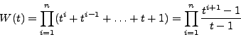
| CPU-time (sec) | |||
| 3 | 0.05 | 24 | 6 |
| 4 | 0.28 | 120 | 10 |
| 5 | 3.04 | 720 | 15 |
| 6 | 40.58 | 5040 | 21 |
| 7 | 633.32 | 40320 | 28 |
| 8 | 11069.00 | 362880 | 36 |
 and change it with identifications into
 ?
?
#call(monomialsum(2,x,y,z) should return
#call(monomialsum() creates the sum of
all monomials in
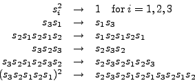
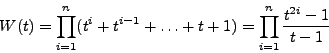
In this section we shall discuss three control structures, known at the compiler level: choice, repetition, and ``go to''.
The preprocessor conditional statement only selects statements for execution;
it does not restrict the set of expressions to be manipulated. For this
purpose, FORM has a ``real'' if statement with the following syntax.
if (condition);
statseq
[elseif (condition);
statseq ]*
[else;
statseq ]
endif;
if (condition);
statement;
endif;
if (condition) statement;
An example:
    Symbols a,b,c;
    Local F = a*c + b*c;
    if (match(a)) id c=a;
    endif;
    Print;
    .end

   F =
      a^2 + b*c;
In the above example, the match function selects only those terms
that have an a inside. Only for these terms, the substitution rule
is applied.
One more example:
    Symbols a,b,c;
    Local F = a*c + b*c;
    if (match(a)=0) id c=a;
    Print;
    .end

   F =
      a*b + a*c;
Now, only those expressions are selected that do not contain an
a. The way it works is that match(expression)
returns the number of times the pattern matches the term. The pattern
is given in the same format as the left-hand side of a substitution. So it
may contain keywords like once, many, select, etc.,
and it may contain wildcards.
Three other ``questions about terms'' can be made in FORM:
count(object, weight, ) counts the
number of times the object occurs with given weight in the current
term.
coefficient return the numerical coefficient of the current term.
findLoop returns the value 1 if a certain loop exists in the
current term, and 0 otherwise. A loop is a cyclic contraction of summable
indices in (anti)symmetric functions or tensors. Examples of loops of
size 3 aref(i1,i2)*f(i2,i3)*f(i3,i1) and
f(i4,i1,i2)*f(i5,i2,i3)*f(i6,i3,i1)*f(i4,i7,i8).
The count function is for power counting.
In the example below, we use it to get rid of all terms of a polynomial
of too high degree.
    Symbols x;
    Local F = 1 + x + x^2 + x^3 + x^4 + x^5 + x^6;
    if (count(x,1)>3) discard;
    endif;
    Print;
    .end

   F =
      1 + x + x^2 + x^3;
The second argument of count is the weight of the first object.
You can have weights different from the usual number 1. The next example
illustrates that when x has weight 2, the term x^2 has a power
counted as 4 and therefore can be discarded.
    Symbols x;
    Local F = 1 + x + x^2 + x^3 + x^4 + x^5 + x^6;
    if (count(x,2)>3) discard;
    Print;
    .end

   F =
      1 + x;
One can also test whether the exponent of a monomial
is a multiple of a given number. For example, the statement
if ( count(x,1) = multipleof(3) )
tests whether the exponent of a monomial in x is a multiple of 3.
    Symbols x;
    Local F = 1 + x + x^2 + x^3 + x^4 + x^5 + x^6;
    if (count(x,1)=multipleof(3)) discard;
    Print;
    .end

   F =
      x + x^2 + x^4 + x^5;
coefficient, which is also abbreviated as
coeff, returns the numeric coefficient of the current term. It can for
instance be used to discard terms with too small coefficients.
    Symbols a,b,i,j;
    Local F = sum_(i,0,4,a^i/fac_(i)) * sum_(j,0,4,b^j/fac_(j));
    if (coefficient < 1/10) discard;
    Bracket b;
    Print;
    .end

   F =
       + b * ( 1 + a + 1/2*a^2 + 1/6*a^3 )

       + b^2 * ( 1/2 + 1/2*a + 1/4*a^2 )

       + b^3 * ( 1/6 + 1/6*a )

       + 1 + a + 1/2*a^2 + 1/6*a^3;
In the first chapter, in subsection 1.4.6, we have used
the symmetric dd_ function to find graphs with prescribed
degrees. For FORM to be more useful in graph theory, it must provide
ways to detect and manipulate cycles or loops in graphs, i.e., paths in
graphs with common begin- and endpoint. The FORM functions replaceLoop
and findLoop serve this purpose in the context of (anti)symmetric
functions or tensors with summable indices.
We give a simple example to illustrate the syntax and use of findLoop:
we determine all connected, loop-free graphs with degree sequence
1,1,2,2,3,3 and without multiple edges or loops of size 3.
    AutoDeclare Vector v;
    AutoDeclare Index i;
    CTensor f(symmetric);
    Local G = dd_(v1,v2,v3,v3,v4,v4,v5,v5,v5,v6,v6,v6);
    id v?.v?=0;     * loop-free
    id v1?.v2?^2=0; * no multiple edges
    id v1.v2=0;     * connected
    Format 65;
    Print;
    .sort

   G =
      144*v1.v3*v2.v5*v3.v6*v4.v5*v4.v6*v5.v6 + 144*v1.v3*v2.v6*
      v3.v5*v4.v5*v4.v6*v5.v6 + 144*v1.v4*v2.v5*v3.v5*v3.v6*
      v4.v6*v5.v6 + 144*v1.v4*v2.v6*v3.v5*v3.v6*v4.v5*v5.v6 +
      144*v1.v5*v2.v3*v3.v6*v4.v5*v4.v6*v5.v6 + 144*v1.v5*v2.v4*
      v3.v5*v3.v6*v4.v6*v5.v6 + 144*v1.v5*v2.v5*v3.v4*v3.v6*
      v4.v6*v5.v6 + 144*v1.v5*v2.v6*v3.v4*v3.v5*v4.v6*v5.v6 +
      144*v1.v5*v2.v6*v3.v4*v3.v6*v4.v5*v5.v6 + 144*v1.v5*v2.v6*
      v3.v5*v3.v6*v4.v5*v4.v6 + 144*v1.v6*v2.v3*v3.v5*v4.v5*
      v4.v6*v5.v6 + 144*v1.v6*v2.v4*v3.v5*v3.v6*v4.v5*v5.v6 +
      144*v1.v6*v2.v5*v3.v4*v3.v5*v4.v6*v5.v6 + 144*v1.v6*v2.v5*
      v3.v4*v3.v6*v4.v5*v5.v6 + 144*v1.v6*v2.v5*v3.v5*v3.v6*
      v4.v5*v4.v6 + 144*v1.v6*v2.v6*v3.v4*v3.v5*v4.v5*v5.v6;

    repeat;
      #do l=1,6
        #do k=1,`l'
           id v`k'.v`l' = f(i`k',i`l');
        #enddo
      #enddo
    endrepeat;
    if (findLoop(f,arguments=2,loopsize=3)) discard;
    repeat;
      #do l=1,6
        #do k=1,`l'
           id f(i`k',i`l') = v`k'.v`l';
        #enddo
      #enddo
    endrepeat;
    Print;
    .end

   G =
      144*v1.v5*v2.v6*v3.v4*v3.v5*v4.v6*v5.v6 + 144*v1.v5*v2.v6*
      v3.v4*v3.v6*v4.v5*v5.v6 + 144*v1.v5*v2.v6*v3.v5*v3.v6*
      v4.v5*v4.v6 + 144*v1.v6*v2.v5*v3.v4*v3.v5*v4.v6*v5.v6 +
      144*v1.v6*v2.v5*v3.v4*v3.v6*v4.v5*v5.v6 + 144*v1.v6*v2.v5*
      v3.v5*v3.v6*v4.v5*v4.v6;
From the expression G in the two stages of the computation it is
clear that graphs of type
have been removed and that we are left with graphs of type
In the second stage of the above computation, we first rewrite
the dot products of vectors in terms of function calls of the symmetric
functions f with the indices corresponding with the vectors.
In the conditional statement, if a term is encountered that is a loop of
size 3 in the function calls of f with 2 arguments,
then this term is discarded.
Hereafter we rewrite the product of function calls as dot products of vectors.
These terms represent the graphs that are left.
We have used one of the allowed formats of the findLoop
statement:
findLoopfunction,arguments=number,loopsize=number
where function is a symmetric or antisymmetric function or tensor.
The arguments part says that only occurrences of the function with
the specified number of arguments are considered.
The loopsize part says that only loops of certain size are considered;
in our example, only loops of size 3.
Other options are loopsize<number, in which case all loops of
size less than the specified number are considered, and
loopsize=all, in which case all loops are considered.
So, we could have left out the id v1?.v2?^2=0; and instead we could
have used the condition loopsize<4 to obtain the same result.
You can also specify via the option include=index which summable
index must be included in the loop. The order of the option is irrelevant.
The replaceLoop statement has one more mandatory argument, viz.,
outfun=name, in which the name of the (cyclesymmetric)
function is given that is used to collect the remaining indices.
For example,
replaceLoop f,arguments=3,loopsize=3,outfun=ff;replaces
f(i4,i1,i2)*f(i5,i2,i3)*f(i6,i3,i1)*f(i4,i7,i8)by
f(i4,i5,i6)*f(i4,i7,i8),but the statement
replaceLoop f,arguments=3,loopsize=3,outfun=ff,include=i9;leaves the term as it is.
Let us continue with the discussion about the conditional statement at compiler level. As we have seen in the previous section, relational operators are in FORM mostly the same as in the C programming language. The same holds for logical operators with the exception that the negation (! in C) does not exist in FORM.
| Operator | Meaning |
| = or == | equal to |
| != | not equal to |
| greater than | |
| less than | |
| greater than or equal to | |
| less than or equal to | |
| && | and |
| or |
Furthermore, the conditional statement must be completely within a
single module; one cannot have a .sort statement inside an
if-statement.
The same holds for other control sturctures at compiler level such
as the repetition constructs repeat and while,
which will be discussed in the next subsection.
Repetitions can be constructed in several ways. You have already seen the
repeat statement in several examples.
Its syntax is
repeat;
statseq
endrepeat;
while-loop, which has the following syntax.
while (condition);
statseq
endwhile;
    Symbols x,y,z;
    Local F = x^3 * y^5;
    while ( match(x*y^2) );
      id x*y^2 = z;
    endwhile;
    print;
    .end

   F =
      x*y*z^2;
So, the replacement rule
Another way to construct loops is by labels and goto-statements.
Below is an example of a post-checked repetition.
    Symbols x;
    Local F = 1;
    Label 1;
    Multiply x;
    if (count(x,1)<10);
       goto 1;
    endif;
    print;
    .end;

   F =
      x^10;
The prototype of this post-checked repetition is as follows:
label 1;
statseq
if (condition);
goto 1;
endif;
label 1;
if (condition);
statseq
goto 1;
endif;
    Symbols x,y;
    Local F = 1 + y^2*x^4 + y^3*x^5 + y^4*x^6 + y^5*x^7;
    if (count(y,-1,x,2)>7);
       discard;
    endif;
    Print;
    .end
 and then
throw away all terms with positive exponent and those with coefficient
smaller than
and then
throw away all terms with positive exponent and those with coefficient
smaller than
 .
.
Local [(a+b)^2] = (a+b)^2 statement
in the first example by Local [(a+b)^2] = (a+b)*(a+b) ?
The proof is in eating the pudding.
    FORM version 3.-(Nov 29 1997). Run at: Tue Jan  6 19:32:18 1998
    Symbols a,b;
    Local [(a+b)^2] = (a+b)^2;
    Print;
    .end
Time =       0.10 sec    Generated terms =          3
                F        Terms in output =          3
                         Bytes used      =         52
    [(a+b)^2] =
       2*a*b + a^2 + b^2;
FORM recognizes the equal terms in the product and treats them as
powers so that the binomial formula of Newton can be applied instead
of working out the brackets one by one. This is one of the rare
cases in which FORM touches the input. In general, FORM never
tries to interpret the right hand side of a statement until it needs
it and even then it is inserted in its proper place before any
interpretation takes place.
Symbols a,b
declaration in the first example by
Functions a,b ?
The FORM session:
    FORM version 3.-(Nov 29 1997). Run at: Tue Jan 6 19:42:14 1998
    Functions a,b;
    Local F = (a+b)^2;
    Print;
    .end
Time =       0.10 sec    Generated terms =          4
                F        Terms in output =          4
                         Bytes used      =         74

   F =
      a*a + a*b + b*a + b*b;
Here, a and b are used as functions (without arguments).
A general property of functions in FORM is that they do not commute.
Hence, the binomial formula of Newton cannot be applied.
The brackets must be worked out by brute force into a sum of 4 terms.
    Symbol a;
    Functions b, c;
    Local F1 = (a+b+c)^2;
    Local F2 = (a+(b+c))^2;
    Print;
    .end;
What is the difference in working out expression F1 and expression
F2?
The FORM session:
    FORM version 3.-(Nov 29 1997). Run at: Wed Jan  7 13:04:18 1998
    Symbol a;
    Functions B, C;
    Local F1 = (a+B+C)^3;
    Local F2 = (a+(B+C))^3;
    Print;
    .end;
Time =       0.16 sec    Generated terms =         27
               F1        Terms in output =         15
                         Bytes used      =        286

Time =       0.27 sec    Generated terms =         15
               F2        Terms in output =         15
                         Bytes used      =        286

   F1 =
      a^3 + 3*B*a^2 + 3*B*B*a + B*B*B + B*B*C + 3*B*C*a + B*C*B + B*C*C + 3*C*
      a^2 + 3*C*B*a + C*B*B + C*B*C + 3*C*C*a + C*C*B + C*C*C;

   F2 =
      a^3 + 3*B*a^2 + 3*B*B*a + B*B*B + B*B*C + 3*B*C*a + B*C*B + B*C*C + 3*C*
      a^2 + 3*C*B*a + C*B*B + C*B*C + 3*C*C*a + C*C*B + C*C*C;
Note that the expansion of expression F1 needs more intermediate
terms. The reason is the following:
both expressions contain one symbol and two functions, in other
words one commuting and two noncommuting objects.
The rule that is used by FORM is that binomial expansion is
applicable when at most one noncommuting object is involved.
Therefore, expression F1 must be expanded by brute force, which
generates some extra intermediate terms. In expression F2, the
noncommuting functions are grouped into a single noncommuting
object. Hence, the third power can be expanded first by the binomial
formula of Newton into a sum of four terms. Hereafter the powers
of B+C are worked out.
You may wonder why FORM does not automatically place brackets, but
this would violate the principle of not touching the input if not necessary.
    s,t,u; * these are the symbols to be used.
    L,F =
    (t+u)
    ^2;    * this is the local expression to be manipulated.
    Print; .end
The following FORM session shows that there are no difficulties.
    FORM version 3.-(Nov 29 1997). Run at: Wed Jan  7 13:00:59 1998
    s,t,u; * these are the symbols to be used.
    L,F =
    (t+u)
    ^2;    * this is the local expression to be manipulated.
    Print; .end

Time =       0.01 sec    Generated terms =          3
                F        Terms in output =          3
                         Bytes used      =         52

   F =
      2*t*u + t^2 + u^2;
In the FORM session below you see examples of the Einstein summation convention and of the SCHOONSCHIP notation.
    Vectors x,y;
    Tensor a;
    Indices i,j;
    Local F1 = a(i,j)*x(j);
    Local F2 = a(i,i)*x(j);
    Local F3 = a(i,j)*x(i)*y(j);
    Local F4 = d_(i,j)*x(i)*x(j);
    Print;
    .end

   F1 =
      a(i,x);

   F2 =
      a(i,i)*x(j);

   F3 =
      a(x,y);

   F4 =
      x.x;
We show that the difference of left- and right-hand side of the equations are equal to zero. Automatic contraction will do the work.
    Vectors x,y;
    Tensor a;
    Indices i,j;
    Local F1 = a(i,j)*x(i)*y(j) - a(j,i)*x(j)*y(i);
    Local F2 = (a(i,j) + a(j,i))*x(i)*x(j) - 2*a(i,j)*x(i)*x(j);
    Print;
    .end

   F1 = 0;

   F2 = 0;
The first property is immediately clear in FORM when you
declare the tensor ![]() to be antisymmetric. The second property
is verified by showing that
to be antisymmetric. The second property
is verified by showing that
![]() .
.
    Tensor A(antisymmetric);
    Vectors x;
    Indices i,j,k;
    Local F1 = A(i,j)*x(i)*x(j);
    Local F2 = A(i,k)*A(k,j) - A(j,k)*A(k,i);
    Print;
    .end

   F1 = 0;

   F2 = 0;
   FunPowers nofunpowers;
   FunPowers commutingonly;
   FunPowers allfunpowers;
Find out by experimentation what the statements actually do and check also how they affect the printing of powers of tensors.
First a FORM session that shows everything:
    Function f;
    Commuting g;
    Tensor t;
    Local expr = f*f*g*g*t*t;
    Print;
    .sort;

   expr =
      f*f*g^2*t*t;

    FunPowers nofunpowers;
    Print;
    .sort

   expr =
      f*f*g*g*t*t;

    FunPowers commutingonly;
    Print;
    .sort

   expr =
      f*f*g^2*t*t;

    FunPowers allfunpowers;
    Print;
    .end

   expr =
      f^2*g^2*t*t;
Conclusions:
nofunpowers, products of same functions are never
printed with powers.
commutingonly, products of same commuting functions
are printed with powers and products of same noncommuting functions are not.
This is the default behavior of FORM.
allfunpowers, all products of same functions, regardless
of there type, are printed with powers.
.
    Symbols x,y,i,j;
    CFunction a;
    Local F=sum_(i,0,2,x^i*sum_(j,0,2,a(i,j)*y^j));
    Print;
    .end

   F =
      a(0,0) + a(0,1)*y + a(0,2)*y^2 + a(1,0)*x + a(1,1)*x*y + a(1,2)*x*y^2 +
      a(2,0)*x^2 + a(2,1)*x^2*y + a(2,2)*x^2*y^2;
sump_.
It works like the regular function sum_, except
that the last argument is not the sump_(i,0,10,x) evaluates
to the series expansion of
Use the function sump_ to compose the
expression
,
and write it as a polynomial in ![]() .
.
    Symbols x,y,i,j;
    Local F=sump_(i,0,3,x/i)*sump_(j,0,3,y/j);
    Bracket x;
    Print;
    .end

   F =
       + x * ( 1 + y + 1/2*y^2 + 1/6*y^3 )

       + x^2 * ( 1/2 + 1/2*y + 1/4*y^2 + 1/12*y^3 )

       + x^3 * ( 1/6 + 1/6*y + 1/12*y^2 + 1/36*y^3 )

       + 1 + y + 1/2*y^2 + 1/6*y^3;
, but throw away all powers of degree 4 and higher.
In the declaration of a symbol you may already restrict the powers that will appear in the result.
    Symbol i, x(:3);
    Local F = sum_(i,0,10,(x+1)^i);
    Print;
    .end

   F =
      11 + 55*x + 165*x^2 + 330*x^3;
    Vectors p,P;
    Indices mu=0;
    Symbols c,t,x,y,z;
    Local F = p(mu)*P(mu);
    sum mu,0,1,2,3;
    id p(0) = c*t;
    id p(1) = x;
    id p(2) = y;
    id p(3) = z;
    id P(0) = -c*t;
    id P(1) = x;
    id P(2) = y;
    id P(3) = z;
    Print;
    .end

   F =
       - c^2*t^2 + x^2 + y^2 + z^2;
    Dimension 3;
    Vectors A,B,C,D;
    Indices i,j,k,l,m,n,p,q;
    Local F1 = e_(i,j,k)*A(i)*B(j) * e_(m,n,k)*A(m)*B(n);
    Local F2 = e_(i,j,k) * (e_(m,n,i)*A(m)*B(n)) * C(j) -
               e_(i,j,k) * A(i) * (e_(m,n,j)*B(m)*C(n));
    Local F3 = e_(i,j,k) * A(i) * (e_(m,n,j)*B(m)*C(n)) +
               e_(i,j,k) * B(i) * (e_(m,n,j)*C(m)*A(n)) +
               e_(i,j,k) * C(i) * (e_(m,n,j)*A(m)*B(n));
    Local F4 = e_(i,j,k) * (e_(m,n,i)*A(m)*B(n)) * (e_(p,q,j)*C(p)*D(q));
    Local F5 = e_(i,j,k)*(A(i)-B(i))*(A(j)+B(j));
    Local F6 = e_(i,j,k)*A(i)*B(j) * e_(m,n,k)*C(m)*D(n) +
               e_(i,j,k)*B(i)*C(j) * e_(m,n,k)*A(m)*D(n) +
               e_(i,j,k)*C(i)*A(j) * e_(m,n,k)*B(m)*D(n);
    contract;
    Print;
    .end

   F1 =
      A.A*B.B - A.B^2;

   F2 =
       - A(k)*B.C + C(k)*A.B;

   F3 = 0;

   F4 =
      e_(A,C,D)*B(k) - e_(B,C,D)*A(k);

   F5 =
      2*e_(A,B,k);

   F6 = 0;
where there are ![]() lines constructed with the
lines constructed with the ![]() , and
, and ![]() lines constructed
with the
lines constructed
with the ![]() .
The resultant of
.
The resultant of ![]() and
and ![]() , denoted by
, denoted by
![]() ,
or
,
or
![]() if there has to be a
variable
if there has to be a
variable ![]() , is the determinant of the Sylvester matrix.
The importance of the resultant lies in the following theorem.
, is the determinant of the Sylvester matrix.
The importance of the resultant lies in the following theorem.
(i) Consider the polynomial ![]() . To find common zeros
of the polynomial
. To find common zeros
of the polynomial ![]() and its derivate
and its derivate ![]() , we need to work out
the condition
, we need to work out
the condition
![]() . Note that in this case
. Note that in this case
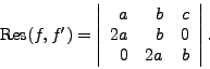
    Symbols a,b,c,x;
    CFunction M;
    Indices i1,i2,i3;
    Local R = e_(1,2,3)*e_(i1,i2,i3)*M(1,i1)*M(2,i2)*M(3,i3);
    contract;
    id M(1,1) = a;
    id M(1,2) = b;
    id M(1,3) = c;
    id M(2,1) = 2*a;
    id M(2,2) = b;
    id M(2,3) = 0;
    id M(3,1) = 0;
    id M(3,2) = 2*a;
    id M(3,3) = b;
    Print;
    .end

   R =
       - a*b^2 + 4*a^2*c;
We get
(ii) Consider the polynomial
![]() . To find discriminant
of
. To find discriminant
of ![]() , we use the formula
, we use the formula
![]() .
Note that in this case
.
Note that in this case
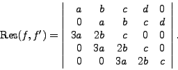
    Symbols a,b,c,d,x;
    CFunction M;
    AutoDeclare Indices i;
    Local D = - e_(1,2,3,4,5)*e_(i1,i2,i3,i4,i5)*
              M(1,i1)*M(2,i2)*M(3,i3)*M(4,i4)*M(5,i5) / a;
    contract;
    id M(1,1) = a;
    id M(1,2) = b;
    id M(1,3) = c;
    id M(1,4) = d;
    id M(1,5) = 0;
    id M(2,1) = 0;
    id M(2,2) = a;
    id M(2,3) = b;
    id M(2,4) = c;
    id M(2,5) = d;
    id M(3,1) = 3*a;
    id M(3,2) = 2*b;
    id M(3,3) = c;
    id M(3,4) = 0;
    id M(3,5) = 0;
    id M(4,1) = 0;
    id M(4,2) = 3*a;
    id M(4,3) = 2*b;
    id M(4,4) = c;
    id M(4,5) = 0;
    id M(5,1) = 0;
    id M(5,2) = 0;
    id M(5,3) = 3*a;
    id M(5,4) = 2*b;
    id M(5,5) = c;
    Print;
    .end

   D =
      18*a*b*c*d - 4*a*c^3 - 27*a^2*d^2 + b^2*c^2 - 4*b^3*d;

    AutoDeclare Vectors u,v;
    Symbol a,b,c,d;
    Local det = e_(u1,u2)*e_(v1,v2);
    contract;
    id u1.v1 = a;
    id u1.v2 = b;
    id u2.v1 = c;
    id u2.v2 = d;
    Print;
    .end

   det =
      a*d - b*c;
(i)
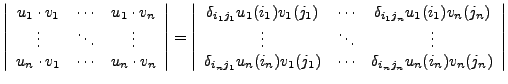
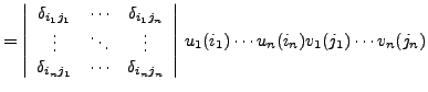
![]()
![]()
(ii)
Below you see the printouts of the computation of a general ![]() matrix with both methods under default settings of FORM and using
a Pentium 166Mhz PC with 16 MB RAM. Most statistics messages have been
left out.
matrix with both methods under default settings of FORM and using
a Pentium 166Mhz PC with 16 MB RAM. Most statistics messages have been
left out.
    *
    * Method with functions
    *
    AutoDeclare Indices i;
    CFunction M;
    On statistics;
    Local detF = e_(1,...,10)*
                 e_(i1,...,i10)*
                 M(1,i1)*M(2,i2)*M(3,i3)*M(4,i4)*M(5,i5)*
                 M(6,i6)*M(7,i7)*M(8,i8)*M(9,i9)*M(10,i10);
    contract;
    .end;

    :
    :
    :

Time =    1208.26 sec    Generated terms =    3628800
             detF        Terms in output =    3628800
                         Bytes used      =  130839812

    *
    * Method with vectors
    *
    AutoDeclare Vectors u,v;
    On statistics;
    Local detV = e_(u1,...,u10)*
                 e_(v1,...,v10);
    contract;
    .end

    :
    :
    :

Time =     410.66 sec    Generated terms =    3628800
             detV        Terms in output =    3628800
                         Bytes used      =   88215006
As you see the method with commuting functions takes about 20 minutes to
generate all 10! = 3,628,800 terms in the determinant,
whereas the method with vectors only takes 7 minutes.
Also the memory usage of the second method is less because less sorting
is needed.
dd_ in graph theoretical enumeration problems.
dd_.
(i) In the session below the three graphs with requested properties are calculated.
    AutoDeclare Vectors v;
    Local F = dd_(v1,v1,v1,v1,
                  v2,v2,v2,
                  v3,v3,
                  v4);
    id v?.v?=0;        * loop-free
    Print +s F;
    .end

   F =
       + 144*v1.v2^2*v1.v3*v1.v4*v2.v3
       + 72*v1.v2^2*v1.v3^2*v2.v4
       + 48*v1.v2^3*v1.v3*v3.v4
      ;
(ii) The following session proves that no graph with requested properties exists.
    AutoDeclare Vectors v;
    Local F = dd_(v1,v1,v1,v1,v1,v1,v1,
                  v2,v2,v2,v2,v2,
                  v3,v3,v3,v3,
                  v4,v4,v4,
                  v5,v5,
                  v6,v7,v8);
    id v?.v?=0;        * loop-free
    id v1?.v2?^2 = 0;  * no multiple edges
    Print F;
    .end

   F = 0;
(iii) In the session below the one graph with requested properties are calculated.
    AutoDeclare Vectors v;
    Local F = dd_(v1,v1,v1,v1,v1,v1,v1,
                  v2,v2,v2,v2,
                  v3,v3,v3,
                  v4,v4,v4,
                  v5,v5,
                  v6,v7,v8);
    id v?.v?=0;        * loop-free
    id v1?.v2?^2 = 0;  * no multiple edges
    format 65;
    Print F;
    .end

   F =
      8709120*v1.v2*v1.v3*v1.v4*v1.v5*v1.v6*v1.v7*v1.v8*v2.v3*
      v2.v4*v2.v5*v3.v4;
(iv) The session below differs from the ones we already met in this exercises that identify statements are added that are necessary to guarantee connectedness of the graph. They turn out to be sufficient as well.
    AutoDeclare Vectors u,v,w;
    Local F = dd_(u,u,u,v,v,w,w,v1,v2,v3);
    id v?.v?=0;     * loop-free
    id u?.v?^2 = 0; * no multiple edges
    id v1.v2 = 0;   * connected
    id v1.v3 = 0;
    id v2.v3 = 0;
    Print +s F;
    .end

   F =
       + 24*u.v*u.w*u.v1*v.v2*w.v3
       + 24*u.v*u.w*u.v1*v.v3*w.v2
       + 24*u.v*u.w*u.v2*v.v1*w.v3
       + 24*u.v*u.w*u.v2*v.v3*w.v1
       + 24*u.v*u.w*u.v3*v.v1*w.v2
       + 24*u.v*u.w*u.v3*v.v2*w.v1
       + 24*u.v*u.v1*u.v2*v.w*w.v3
       + 24*u.v*u.v1*u.v3*v.w*w.v2
       + 24*u.v*u.v2*u.v3*v.w*w.v1
       + 24*u.w*u.v1*u.v2*v.w*v.v3
       + 24*u.w*u.v1*u.v3*v.w*v.v2
       + 24*u.w*u.v2*u.v3*v.w*v.v1
      ;
It is easy to see that up to isomorphism there is only one graph. The above
graphs are all isomorphic tou.v*u.w*u.v1*v.v2*w.v3 via a permutation of v1, v2,
v3, in combination with a permutation of v and w.
(v) Comparison of the following FORM program would show that the use of
the dd_ function is more efficient. By the way, only the value
of the preprocessor variable `n' has to be changed in the program
listed below.
#define n "10";
Vectors v1,...,v`n';
Local G`n' = e_(v1,...,v`n')^2;
contract;
.end
versus
#define n "10";
Autodeclare Vector v;
Local F = dd_(<v1,v1>,...,<v`n',v`n'>);
.end
. Express
Straightforward substitution does the work.
    Symbols m,a,p,t,v;
    Local T = p^2/(2*m);
    id p = m*v;
    Print;
    .sort

   T =
      1/2*m*v^2;

    id v = a*t;
    Print;
    .end

   T =
      1/2*m*a^2*t^2;
into
In this exercise you only have to take into account differences between
patterns of type x and 1/x, where x is some symbol.
    Symbols x,y;
    Local F1 = x^2 + x + 1/x;
    id x = y;
    id 1/x = 1/y;
    Print F1;
    .sort

   F1 =
      y^-1 + y + y^2;

    Local F2 = x^2 + x + 1/x;
    id x = y;
    Print F2;
    .sort

   F2 =
      x^-1 + y + y^2;

    Local F3 = x^2 + x + 1/x;
    id 1/x = y;
    Print F3;
    .end

   F3 =
      x + x^2 + y;
The trick is to replace a by d-b instead of trying to
replace a+b by d.
    Symbols a,b,c,d;
    Local F = a + b + c;
    id a = d - b;
    Print;
    .end

   F =
      c + d;
Writing the substitution as ![]() will replace all higher powers
of
will replace all higher powers
of x.
    Symbols x,y;
    Local F = (x^2+1)^2 + x^2 + 2;
    id x^2 = y - 1;
    Print;
    .end

   F =
      1 + y + y^2;
In one repeat-loop we shall work out products into canonical form.
    Functions i,j,k;
    Symbols t,u;
    Local F = (u+3*i-k)^3*(-1+t*j);
    repeat;
      id i*j = k;
      id j*k = i;
      id k*i = j;
      id j*i = -k;
      id i*k = -j;
      id k*j = -i;
      id i*i = -1;
      id j*j = -1;
      id k*k = -1;
    endrepeat;
    Bracket i,j,k;
    Print;
    .end

   F =
       + i * ( 30 + 3*t*u^2 - 10*t - 9*u^2 )

       + j * (  - 30*t*u + t*u^3 )

       + k * (  - 10 + 9*t*u^2 - 30*t + 3*u^2 )

       + 30*u - u^3;
The Bracket statement has been added to increase readability.
The trick of augmenting a formula with some extra factor, carrying out operations defined in terms of this extra factor, and finally removing this extra factor, can be applied in many cases. Computing with differential operators to calculate a derivative is just one of the examples.
    Functions D,x,[sin(x)],[cos(x)];
    FunPowers allfunpowers;
    Local F = D^3*x^3*[sin(x)]^2*[cos(x)];
    Print;
    .sort

   F =
      D^3*x^3*[sin(x)]^2*[cos(x)];

    repeat;
      id D*x = x*D + 1;
      id D*[sin(x)] = [sin(x)]*D + [cos(x)];
      id D*[cos(x)] = [cos(x)]*D - [sin(x)];
    endrepeat;
    id D = 0;
    *
    * write all terms in the order of
    * power of x, power of sin(x), power of cos(x).
    *
    repeat;
      id [sin(x)]*x = x*[sin(x)];
      id [cos(x)]*x = x*[cos(x)];
      id [cos(x)]*[sin(x)] = [sin(x)]*[cos(x)];
    endrepeat;
    Print;
    .end

   F =
      7*x^3*[sin(x)]^3 - 20*x^3*[sin(x)]*[cos(x)]^2 - 63*x^2*[sin(x)]^2*
      [cos(x)] + 18*x^2*[cos(x)]^3 - 18*x*[sin(x)]^3 + 36*x*[sin(x)]*[cos(x)]^
      2 + 6*[sin(x)]^2*[cos(x)];
.
do not form a
Lie algebra.
In the FORM program below, D denotes the differential
operator
![]() . All we need to do is repeatedly
use the commutation relation
. All we need to do is repeatedly
use the commutation relation
![$\displaystyle[\frac{d}{dx},x] = 1$](img638.png) to move
the differential operator the right-hand side of expressions.
to move
the differential operator the right-hand side of expressions.
    Functions x,D;
    Symbols a,b,c;
    FunPowers allfunpowers;
    *
    * (i) The requested commutation relations
    *
    Local [D,x*D] = D*x*D - x*D*D;
    Local [D,x^2*D] = D*x^2*D - x^2*D*D;
    Local [x*D,x^2*D] = x*D*x^2*D - x^2*D*x*D;
    repeat;
      id D*x = x*D + 1;
    endrepeat;
    Print;
    .sort

   [D,x*D] =
      D;

   [D,x^2*D] =
      2*x*D;

   [x*D,x^2*D] =
      x^2*D;

    *
    * (ii) The center of the Lie algebra
    *
    Local Z = a*D + b*x*D + c*x^2*D;
    Local [Z,D] = Z*D - D*Z;
    Local [Z,x*D] = Z*x*D - x*D*Z;
    Local [Z,x^2*D] = Z*x^2*D - x^2*D*Z;
    repeat;
      id D*x = x*D + 1;
    endrepeat;
    Print [Z,D], [Z,x*D],[Z,x^2*D];
    .sort

   [Z,D] =
       - 2*x*D*c - D*b;

   [Z,x*D] =
       - x^2*D*c + D*a;

   [Z,x^2*D] =
      x^2*D*b + 2*x*D*a;

    *
    * (iii) Proof that [x^2*D, x^3*D] = x^4*D
    *
    Local [x^2*D,x^3*D] = x^2*D*x^3*D - x^3*D*x^2*D;
    repeat;
      id D*x = x*D + 1;
    endrepeat;
    Print [x^2*D,x^3*D];
    .end

   [x^2*D,x^3*D] =
      x^4*D;
You see that the center of the Lie algebra is equal to 0 because the
system of equations that
Because noncommutative algebra is the default choice in FORM, the system is very convenient for this kind of computations.
    Functions h,e,f;
    FunPowers allfunpowers;
    Local F1 = f^3*e^2*h;
    Local F2 = h * h*e^2*f^3 - h*e^2*f^3 * h;
    repeat;
      id e*h = h*e - 2*e;
      id f*h = h*f + 2*f;
      id f*e = e*f - h;
    endrepeat;
    Print;
    .end

   F1 =
      6*h^3*f - 6*h^2*e*f^2 + 30*h^2*f + h*e^2*f^3 - 18*h*e*f^2 + 48*h*f + 2*e
      ^2*f^3 - 12*e*f^2 + 24*f;

   F2 =
       - 2*h*e^2*f^3;
x, n, explain what the
following patterns mean.
x
1/x
x?
x^n?
x?^n
x?^n?
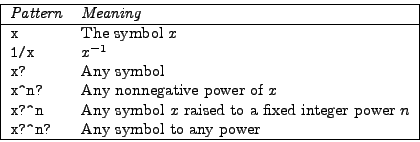
u, v and the indices i,
j, explain what the
following patterns mean.
u(i)
u(i?)
u?(i)
u?(i?)
u(i?)*v(j?)
u(i?)*v(i?)
u.v?
u?.v?
v?.v?
u?.v?^2
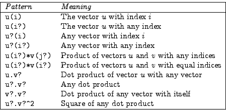
    Symbol x,y;
    Functions odd, even;
    Local ODD = odd(-x);
    Local EVEN = even(-x);
    Local F = odd(-x-y) + even(-x-y) + odd(x-y) + odd(-x+y);
    id odd(-x?) = - odd(x);
    id even(-x?) = even(x);
    Print;
    .end

   ODD =
       - odd(x);

   EVEN =
      even(x);

   F =
      odd( - x - y) + odd( - x + y) + odd(x - y) + even( - x - y);
We added the expression F to illustrate how rudimentary our
current implementation is.
A repeat-loop is necessary to simplify results as far as possible.
    CFunction exp;
    Symbols x,y,a,b,c;
    Local F = (exp(a) + exp(b) + exp(c))^3;
    id exp(x?) * exp(y?) = exp(x+y);
    Print +s;
    .sort;

   F =
       + exp(a)*exp(2*a)
       + 3*exp(b)*exp(a + b)
       + 3*exp(b)*exp(2*a)
       + exp(b)*exp(2*b)
       + 6*exp(c)*exp(a + b)
       + 3*exp(c)*exp(a + c)
       + 3*exp(c)*exp(2*a)
       + 3*exp(c)*exp(b + c)
       + 3*exp(c)*exp(2*b)
       + exp(c)*exp(2*c)
      ;

    repeat;
      id exp(x?) * exp(y?) = exp(x+y);
    endrepeat;
    Print +s;
    .end

   F =
       + 6*exp(a + b + c)
       + 3*exp(a + 2*b)
       + 3*exp(a + 2*c)
       + 3*exp(2*a + b)
       + 3*exp(2*a + c)
       + exp(3*a)
       + 3*exp(b + 2*c)
       + 3*exp(2*b + c)
       + exp(3*b)
       + exp(3*c)
      ;
All you need to do is to write the substitution rule in the form of
![]() .
.
    CFunctions sin, cos;
    Symbols a,x;
    Local F1 = sin(a)^2 - 1;
    Local F2 = sin(a)^3;
    id sin(x?)^2 = 1 - cos(x)^2;
    Bracket sin;
    Print;
    .end

   F1 =
       - cos(a)^2;

   F2 =
       + sin(a) * ( 1 - cos(a)^2 );
We shall give two solutions to the problem: one simple, but inefficient program, and another more complicated program that works much more efficient.
    *
    * easy, but inefficient program
    *
    Symbols a,x,n;
    CFunction L;
    On statistics;
    Local Laguerre8 = L(8,a,x);
    repeat;
      id L(1,a,x) = 1;
      id L(2,a,x) = 1+a-x;
      id L(n?,a,x) = (2*n+a-1-x)/n*L(n-1,a,x) - (n+a-1)/n*L(n-2,a,x);
    endrepeat;
    Print;
    .end

Time =      11.83 sec    Generated terms =      20000
        Laguerre8      1 Terms left      =         35
                         Bytes used      =        492

Time =      19.02 sec    Generated terms =      32181
        Laguerre8      1 Terms left      =         70
                         Bytes used      =        984

Time =      19.03 sec    Generated terms =      32181
        Laguerre8        Terms in output =         36
                         Bytes used      =        508

   Laguerre8 =
      1 - 1389/140*a*x + 76529/10080*a*x^2 - 1507/672*a*x^3 +
      295/1008*a*x^4 - 17/1008*a*x^5 + 1/2880*a*x^6 + 481/140*a
       - 381/80*a^2*x + 50177/20160*a^2*x^2 - 9883/20160*a^2*x^3
       + 157/4032*a^2*x^4 - 1/960*a^2*x^5 + 349/144*a^2 - 5953/
      5040*a^3*x + 8129/20160*a^3*x^2 - 1/21*a^3*x^3 + 1/576*a^3
      *x^4 + 329/360*a^3 - 467/2880*a^4*x + 131/4032*a^4*x^2 - 1/
      576*a^4*x^3 + 115/576*a^4 - 59/5040*a^5*x + 1/960*a^5*x^2
       + 73/2880*a^5 - 1/2880*a^6*x + 1/576*a^6 + 1/20160*a^7 -
      7*x + 2441/280*x^2 - 3187/840*x^3 + 247/336*x^4 - 347/5040
      *x^5 + 61/20160*x^6 - 1/20160*x^7;

    *
    * less obvious, but efficient program
    *
    Symbols a, x, n, last, secondlast, dummy;
    CFunction L;
    On statistics;
    Local Laguerre8 = L(2,1+a-x,1)*dummy^6;
    repeat;
      id L( n?, last?, secondlast?) * dummy =
         L( n+1, (2*n+a+1-x)/(n+1)*last - (n+a)/(n+1)*secondlast, last );
    endrepeat;
    id L( n?, last?, secondlast? ) = last;
    .end

Time =       0.29 sec    Generated terms =         36
        Laguerre8        Terms in output =         36
                         Bytes used      =        508
    Symbols x,dx,n;
    *
    * Next could be any polynomial in x
    *
    Local P = 1+x+x^3;
    *
    * Tag the expression and apply differentiation rule
    *
    multiply dx;
    id dx*x^n? = 1/(n+1)*x^(n+1);
    Print;
    .end

   P =
      x + 1/2*x^2 + 1/4*x^4;
Below, we use uppercase characters X, Y, Z, and
T to denote the new coordinates ![]() .
.
    Symbols t, x, y, z, v, c, gamma, [c^2-v^2];
    Local X = gamma*(x-v*t);
    Local Y = y;
    Local Z = z;
    Local T = c*gamma*(t-v*x/c^2);
    Local S = X^2 + Y^2 + Z^2 - T^2;
    id gamma^2 = c^2/[c^2-v^2];
    repeat;
      id c^2/[c^2-v^2] = 1 + v^2/[c^2-v^2];
    endrepeat;
    Print S;
    .end

   S =
       - t^2*c^2 + x^2 + y^2 + z^2;
.
FORM is not good in working with rational expressions: you have to
write the denominator as one function, say [1-phi(n)^2],
and then design appropriate rewrite rules for getting the job
done. Another point in the program below is that for computing derivates
we need to work with noncommuting objects. This is why we distinguish
between commuting and noncommuting functions. Uppercase characters are
used to denote commuting functions; corresponding names in lowercase
refer to the corresponding noncommuting functions.
    Functions g, ginv, del, phi, [1-phi(n)^2];
    CFunctions PHI, [1-PHI(n)^2];
    FunPowers allfunpowers;
    Indices i,j,k,l,n;
    *
    * (i) metric tensor and its inverse
    *
    Local [g(ik)] = d_(i,k) + PHI(i)*PHI(k)/[1-PHI(n)^2];
    Local [ginv(kj)] = d_(k,j) - PHI(k)*PHI(j);
    Local I = [g(ik)] * [ginv(kj)];
    id PHI(i?)^2 = 1 - [1-PHI(n)^2];
    id 1/PHI? * PHI? = 1;
    Print I;
    .sort

   I =
      d_(i,j);

    *
    * (ii) Christoffel symbols of the 1st kind
    *
    Local C1 = 1/2*( del(k)*g(j,l) + del(j)*g(l,k) - del(l)*g(j,k));
    *
    * definition of metric tensor
    *
    id g(i?,j?) = d_(i,j) + phi(i)*phi(j)/[1-phi(n)^2];
    *
    * rules for differentiation
    *
    repeat;
      id del(i?)*phi(j?) = d_(i,j)+ phi(j)*del(i);
    endrepeat;
    id del(i?)/[1-phi(n)^2] = 2*phi(i)/[1-phi(n)^2]^2;
    id del(i?) = 0;
    Print +s C1;
    .sort;

   C1 =
       - phi(j)*phi(k)*phi(l)*([1-phi(n)^2])^(-2)
       + phi(j)*phi(l)*phi(k)*([1-phi(n)^2])^(-2)
       + phi(l)/([1-phi(n)^2])*d_(j,k)
       + phi(l)*phi(k)*phi(j)*([1-phi(n)^2])^(-2)
      ;

    *
    * normalization:
    *   bring over one denominator = (1-phi(n)^2)^2
    *   first we simplify the numerator
    *
    id 1/[1-phi(n)^2]^2 = 1;
    id 1/[1-phi(n)^2] = 1-phi(n)^2;
    *
    * move to commuting functions
    *
    id phi(i?) = PHI(i);
    *
    * further simplification of numerator
    *
    id PHI(i?)^2 = 1 - [1-PHI(n)^2];
    *
    * The requested formula
    *
    multiply 1/[1-PHI(n)^2]^2;
    id PHI?^(-2) * PHI? = 1/PHI;
    Print +s C1;
    .sort

   C1 =
       + ([1-PHI(n)^2])^(-2)*PHI(j)*PHI(k)*PHI(l)
       + 1/([1-PHI(n)^2])*PHI(l)*d_(j,k)
      ;

    *
    * (iii) Christoffel symbols of 2nd kind
    *
    Local C2 = ginv(i,l) * C1;
    id ginv(i?,j?) = d_(i,j) - PHI(i)*PHI(j);
    Print C2;
    .sort

   C2 =
      ([1-PHI(n)^2])^(-2)*PHI(i)*PHI(j)*PHI(k) - ([1-PHI(n)^2])^(-2)*PHI(i)*
      PHI(j)*PHI(k)*PHI(l)^2 + 1/([1-PHI(n)^2])*PHI(i)*d_(j,k) - 1/(
      [1-PHI(n)^2])*PHI(i)*PHI(l)^2*d_(j,k);

    *
    * normalization:
    *   bring over one denominator = (1-PHI(n)^2)^2
    *   first we simplify the numerator
    *
    id 1/[1-PHI(n)^2]^2 = 1;
    id 1/[1-PHI(n)^2] = 1-PHI(n)^2;
    *
    * further simplification of numerator
    *
    id PHI(i?)^2 = 1 - [1-PHI(n)^2];
    Print +s C2;
    .sort

   C2 =
       + PHI(i)*PHI(j)*PHI(k)*[1-PHI(n)^2]
       + PHI(i)*[1-PHI(n)^2]^2*d_(j,k)
      ;

    *
    * bringing back the denominator
    *
    id [1-PHI(n)^2]*[1-PHI(n)^2] = 1;
    id [1-PHI(n)^2] = 1/[1-PHI(n)^2];
    AntiBracket PHI;
    Print +s C2;
    .end

   C2 =

       + d_(j,k) * (
          + PHI(i)
          )

       + 1/([1-PHI(n)^2]) * (
          + PHI(i)*PHI(j)*PHI(k)
          );
So, we have
We give two solutions to the problem. The first one is a very direct, but somewhat elaborate way of getting the job done.
    Symbols x,y,z,a,b,c,dummy,n;
    CFunction ln;
    Local F1 = ln(a*b);
    Local F2 = ln(a*b*c);
    id ln(x?*y?) = ln(x) + ln(y);
    Print;
    .sort

   F1 =
      ln(a) + ln(b);

   F2 =
      ln(a*b*c);

    argument;
      id a = dummy/b;
    endargument;
    id ln(x?*y?) = ln(x) + ln(y);
    argument;
      id dummy = a*b;
    endargument;
    id ln(x?*y?) = ln(x) + ln(y);
    Print F2;
    .sort

   F2 =
      ln(a) + ln(b) + ln(c);

    Local F3 = ln(a*b^3);
    id ln(x?)=x;
    id x?*y?^n? = x+n*y;
    id x? = ln(x);
    Print F3;

   F3 =
      ln(a) + 3*ln(b);
The second solution is more delicate, but works in many more circumstances.
    Symbols x,y,a,b,c,n;
    Function ln;
    Local F1 = ln(a*b);
    Local F2 = ln(a*b*c);
    Local F3 = ln(a*b^3);
    argument ln;
      multiply left ln;
      repeat;
        id ln*x? = ln(x) + ln;
        id ln(x?)*y? = ln(x);
      endrepeat;
      id ln=0;
    endargument;
    id ln(x?) = x;
    Print;

   F1 =
      ln(a) + ln(b);

   F2 =
      ln(a) + ln(b) + ln(c);

   F3 =
      ln(a) + 3*ln(b);
    Symbol M,A,B,C,n;
    CFunction det;
    FunPowers allfunpowers;
    Local F5 = det(M^5);
    Local F3 = det(A*B*C);
    id det(M?)=M;
    repeat;
      id M?=det(M);
    endrepeat;
    Print;
    .end

   F5 =
      det(M)^5;

   F3 =
      det(A)*det(B)*det(C);
Alternatively:
    Symbol M,A,B,C,n;
    CFunction det;
    FunPowers allfunpowers;
    Local F5 = det(M^5);
    Local F3 = det(A*B*C);
    id det(M?)=M;
    repeat;
      id M?=det(M);
    endrepeat;
    Print;
    .end

   F5 =
      det(M)^5;

   F3 =
      det(A)*det(B)*det(C);
, and that a covariant tensor
.
In the program below t(dx,i,up,dxbar,j,low) denotes
![]() .
.
    Tensors [T_kl],U,V,t;
    Indices i,j,k,l,low,up,dx,dxbar;
    Local [Tbar_ij] = U(i,low)*V(j,low) - V(i,low)*U(j,low);
    id U?(i,low) = t(dx,k,up,dxbar,i,low) * U(k,low);
    id U?(j,low) = t(dx,l,up,dxbar,j,low) * U(l,low);
    id U(k,low) * V(l,low) = [T_kl] + V(k,low)*U(l,low);
    Print;
    .end

   [Tbar_ij] =
      [T_kl]*t(dx,k,up,dxbar,i,low)*t(dx,l,up,dxbar,j,low);
    Tensor a,dummy;
    Vectors x,y,z;
    Indices r,s,t;
    Local expr = a(r,s,t)*x(r)*y(s)*z(t);
    multiply dummy();
    repeat;
      id a(?p,z?)*dummy(?q)=a(?p)*dummy(1,?q)*z(1)+a(?p)*dummy(2,?q)*z(2);
    endrepeat;
    id a()*dummy(?p)=a(?p);
    Format 65;
    Print;
    .end

   expr =
      a(1,1,1)*x(1)*y(1)*z(1) + a(1,1,2)*x(1)*y(1)*z(2) + a(1,2,
      1)*x(1)*y(2)*z(1) + a(1,2,2)*x(1)*y(2)*z(2) + a(2,1,1)*
      x(2)*y(1)*z(1) + a(2,1,2)*x(2)*y(1)*z(2) + a(2,2,1)*x(2)*
      y(2)*z(1) + a(2,2,2)*x(2)*y(2)*z(2);
Of course, in real computations you would use the sum_ statement.
ToVector command replaces a tensor into a product
of vector components. For example,
ToVector t,v replaces
t(m1,m2,m3) by v(m1)*v(m2)*v(m3). Use id statements
to get the same job done.
The following program shows that the ToVector command is present
in FORM for convenience and some efficiency only.
    Tensor t;
    Vector v;
    Indices m1,m2,m3;
    Local F = t(m1,m2,m3);
    repeat;
      id t(m1?,?m) = v(m1)*t(?m);
    endrepeat;
    id t() = 1;
    Print;
    .end

   F =
      v(m1)*v(m2)*v(m3);
for
We shall use as metric tensor ![]() and its inverse
and its inverse ![]() for special relativity the one with sign convention
for special relativity the one with sign convention
![]() and
and
![]() , for
, for ![]() .
Then the full contravariant form
.
Then the full contravariant form ![]() is
is
We work out the expression by expansion of the indices
![]() , and
, and ![]() into
into ![]() ,
, ![]() ,
, ![]() , and
, and ![]() ,
respectively. The indices
,
respectively. The indices ![]() run from 1 to 3. Hereafter
we use the definitions of the field tensors.
run from 1 to 3. Hereafter
we use the definitions of the field tensors.
    Dimension 3;
    CFunctions F(antisymmetric), Ft, L, U, eps(antisymmetric);
    Vector E,B;
    Symbol c;
    Indices mu, nu, rho, sigma, i, j, k, l;
    Local expr1 = F(U(mu),U(nu)) * F(L(mu),L(nu));
    Local expr2 = eps(L(mu),L(nu),L(rho),L(sigma)) *
                  F(U(mu),U(nu)) * F(U(rho),U(sigma));
    *
    * expand mu,nu,rho,sigma into 0,i and 0,j, and 0,k, and 0,l, respectively
    *
    sum mu 0,1;
    sum nu 0,2;
    sum rho 0,3;
    sum sigma 0,4;
    argument;
      id L?(1) = L(i);
      id L?(2) = L(j);
      id L?(3) = L(k);
      id L?(4) = L(l);
    endargument;
    repeat;
      id eps(?a,L(i?),?b) = eps(?a,i,?b);
    endrepeat;
    id eps(0,?a) = e_(?a);
    id eps(?a) = 0;
    Format 65;
    Print;
    .sort

   expr1 =
      F(L(i),L(0))*F(U(i),U(0)) + F(L(j),L(i))*F(U(j),U(i)) + F(
      L(j),L(0))*F(U(j),U(0));

   expr2 =
      F(U(i),U(0))*F(U(l),U(k))*e_(i,k,l) + F(U(j),U(i))*F(U(k),
      U(0))*e_(i,j,k) + F(U(j),U(i))*F(U(l),U(0))*e_(i,j,l) + F(
      U(j),U(0))*F(U(l),U(k))*e_(j,k,l);

    *
    * Apply definitions
    *
    id F(U(0),U(j?)) = - E(j)/c;
    id F(U(i?),U(j?)) = - e_(i,j,B);
    id F(L(0),L(j?)) =  E(j)/c;
    id F(L(i?),L(j?)) = - e_(i,j,B);
    contract;
    Print;
    .end

   expr1 =
       - 2*E.E*c^-2 + 2*B.B;

   expr2 =
      8*E.B*c^-1;
So, the invariants can be written as
 and
and
 .
.
    Symbols z,n;
    Function J;
    Local  [J(-3,z)] = J(-3,z);
    Local  [J(-4,z)] = J(-4,z);
    Local  [J(-n,z)] = J(-n,z);
    Local  [J( 4,z)] = J( 4,z);
    id J(n?neg_, ?z) = (-1)^(-n) * J(-n, ?z);
    Print;
    .end

   [J(-3,z)] =
       - J(3,z);

   [J(-4,z)] =
      J(4,z);

   [J(-n,z)] =
      J( - n,z);

   [J(4,z)] =
      J(4,z);
    Functions M, [dM/dt], dt;
    FunPowers allfunpowers;
    Local F = 1/M * 1/M * 1/M;
    multiply left dt;
    repeat;
      id dt*1/M = -1/M*[dM/dt]*1/M + 1/M*dt;
    endrepeat;
    id dt=0;
    Print;
    .end

   F =
       - 1/(M)^3*[dM/dt]/(M) - 1/(M)^2*[dM/dt]/(M)^2 - 1/(M)*[dM/dt]/(M)^3;
    Symbols x,y,n;
    CFunctions log,g;
    Functions [log],[1/x],f,dx;
    Set commuting:log;
    Set noncommuting:[log];
    Set derivative:[1/x];
    *
    Local expr = x^4*log(x)^2;
    id g?commuting?noncommuting(x) = g(x);
    Multiply left dx;
    repeat;
      id dx*g?noncommuting[n](x) = derivative[n](x)+g(x)*dx;
    endrepeat;
    id dx*x^n? = n*x^(n-1);
    id [1/x](x) = 1/x;
    id f?noncommuting?commuting(x) = f(x);
    *
    Print;
    .end

   expr =
      2*log(x)*x^3 + 4*log(x)^2*x^3;
and
.
We compute the integrals by recursion. The select
option in the id statements makes that these rules are
only applied if after matching of the left-hand side of
an expression no elements of the set fromx are left. So,
the first to rules are only applied if no power of x comes
in front of the trigonometric function.
    Symbols x, y, [sin(x)], [cos(x)], n, dx;
    Set fromx: x, [sin(x)], [cos(x)];
    *
    Local exprcos = x^4*[cos(x)];
    Local exprsin = x^4*[sin(x)];
    Multiply dx;
    repeat;
      id select fromx  dx*[sin(x)] = - [cos(x)];
      id select fromx  dx*[cos(x)] = [sin(x)];
      id select fromx dx*x^n?*[sin(x)] =
          - x^n*[cos(x)] + dx*n*x^(n-1)*[cos(x)];
      id select fromx dx*x^n?*[cos(x)] =
          x^n*[sin(x)] - dx*n*x^(n-1)*[sin(x)];
    endrepeat;
    *
    Format 60;
    Print;
    .end

   exprcos =
       - 24*x*[cos(x)] - 12*x^2*[sin(x)] + 4*x^3*[cos(x)] + x^4*[sin(x)]
       + 24*[sin(x)];

   exprsin =
       - 24*x*[sin(x)] + 12*x^2*[cos(x)] + 4*x^3*[sin(x)] - x^4*[cos(x)]
       - 24*[cos(x)];
The tensor
![]() in a coordinate
system
in a coordinate
system
![]() is related to the tensor
is related to the tensor
![]() in a coordinate
system
in a coordinate
system
![]() by the
transformation equation
by the
transformation equation
xbar(a,up,od,b,low) and
x(a,up,odbar,b,low), respectively.
    Tensors [T^ij_ij], T, x, xbar;
    Indices i, j, k, l, m, p, q, r, s, t, low, up, od, odbar;
    Indices k1,...,k5;
    set orig: i, j, k;
    Local [Tbar^ij_ij](k) = T(i,up,j,up,k,low,i,low,j,low);
    *
    * Create the transformed expression
    *
    id T(?a, i?orig, low, ?b) = x(t, up, odbar, i, low) * T(?a, t, low, ?b);
    id T(?a, i?orig, low, ?b) = x(s, up, odbar, i, low) * T(?a, s, low, ?b);
    id T(?a, i?orig, low, ?b) = x(r, up, odbar, i, low) * T(?a, r, low, ?b);
    id T(?a, i?orig,  up, ?b) = xbar(i, up, od, q, low) * T(?a, q,  up, ?b);
    id T(?a, i?orig,  up, ?b) = xbar(i, up, od, p, low) * T(?a, p,  up, ?b);
    *
    Print;
    .sort

   [Tbar^ij_ij](k) =
      T(p,up,q,up,r,low,s,low,t,low)*x(r,up,odbar,k,low)*x(s,up,odbar,i,low)*
      x(t,up,odbar,j,low)*xbar(i,up,od,p,low)*xbar(j,up,od,q,low);

    *
    * Apply transformation rules
    *
    repeat;
      id x(i?, up, odbar, j?, low) * xbar(j?, up, od, k?, low) = d_(i,k);
    endrepeat;
    id T(i?, up, j?, up, k?, low, i?, low, j?, low) = [T^ij_ij](k);
    *
    Print;
    .end

   [Tbar^ij_ij](k) =
      [T^ij_ij](r)*x(r,up,odbar,k,low);
You see that the quantity transforms like a covariant vector.
We use the same notation as in the previous exercise.
    Tensors U, S, T, x, xbar;
    Indices i, j, k, l, m, p, q, r, s, low, up, od, odbar;
    set orig: i, j, l;
    Local Ubar(i,up,l,low) = S(i,up,j,up) * T(j,low,l,low);
    *
    * Create the transformed expression
    *
    id T(?a, i?orig, low, ?b) = x(s, up, odbar, i, low) * T(?a, s, low, ?b);
    id T(?a, i?orig, low, ?b) = x(r, up, odbar, i, low) * T(?a, r, low, ?b);
    id S(?a, i?orig, up, ?b) = xbar(i, up, od, q, low) * S(?a, q, up, ?b);
    id S(?a, i?orig, up, ?b) = xbar(i, up, od, p, low) * S(?a, p, up, ?b);
    *
    * Apply transformation rules
    *
    repeat;
      id x(i?, up, odbar, j?, low) * xbar(j?, up, od, k?, low) = d_(i,k);
    endrepeat;
    id S(i?, up, j?, up) * T(j?, low, l?, low) = U(i, up, l, low);
    Print;
    .end

   Ubar(i,up,l,low) =
      U(p,up,s,low)*x(s,up,odbar,l,low)*xbar(i,up,od,p,low);
You see that the quantity transforms like a mixed tensor of order two.
        Symbol d;
        Dimension d;
        Indices m1, ..., m10;
        On statistics;
        Local F1 = g_(1,m1,m2,...,m10,m1,m2,...,m10);
        tracen,1;
        .sort

Time =       3.51 sec    Generated terms =      20000
               F1      1 Terms left      =          9
                         Bytes used      =        138

Time =       6.97 sec    Generated terms =      40000
               F1      1 Terms left      =         18
                         Bytes used      =        276

Time =      10.44 sec    Generated terms =      60000
               F1      1 Terms left      =         28
                         Bytes used      =        430

Time =      12.59 sec    Generated terms =      72379
               F1      1 Terms left      =         37
                         Bytes used      =        568

Time =      12.59 sec    Generated terms =      72379
               F1        Terms in output =         10
                         Bytes used      =        154
        id d = d-4;
        Print;
        .end

Time =      12.62 sec    Generated terms =         65
               F1        Terms in output =         11
                         Bytes used      =        182

   F1 =
       - 31023169536 + 38971179008*d - 21328977920*d^2 + 6679521280*d^3 -
      1320732160*d^4 + 171464832*d^5 - 14710080*d^6 + 816960*d^7 - 27840*d^8
       + 520*d^9 - 4*d^10;
    V pi, pf, ki, kf, e, ep;
    S k, kp, [alpha^2/(2*m^2) * (kp/k)^2], m;
    Local C = [alpha^2/(2*m^2) * (kp/k)^2] / 16
            * (g_(1,pf) + m)
            * (g_(1,ep,e,ki)/ki.pi + g_(1,e,ep,kf)/kf.pi)
            * (g_(1,pi) + m)
            * (g_(1,ki,e,ep)/ki.pi + g_(1,kf,ep,e)/kf.pi)
            ;
    trace4,1;
    .sort
    *
    repeat;
      id ki.ki = 0;
      id kf.kf = 0;
      id pi.pi = m^2;
      id pf.pf = m^2;
      id pi.e  = 0;
      id pi.ep = 0;
      id pi.pf = m^2 + ki.kf;
      id pi.ki = m*k;
      id 1/(pi.ki)=1/(m*k);
      id pi.kf = m*kp;
      id 1/(pi.kf)=1/(m*kp);
      id pf.e  = -kf.e;
      id pf.ep = ki.ep;
      id pf.ki =  m*kp;
      id pf.kf = m*k;
      id ki.e  = 0;
      id ki.kf = m*(k-kp);
      id kf.ep = 0;
      id  e.e  = -1;
      id ep.ep = -1;
    endrepeat;
    *
    Bracket [alpha^2/(2*m^2) * (kp/k)^2];
    Format 60;
    Print;
    .end

   C =
       + [alpha^2/(2*m^2)*(kp/k)^2] * (  - 1 + 1/2*k^-1*kp
          + 1/2*k*kp^-1 + 2*e.ep^2 );
    Indices mu,nu;
    Vectors a,b;
    CFunction sin,cos;
    Local expr1 = sin(a+b);
    id sin(nu?)=sin(nu)*cos(nu);
    id sin?(?x)*cos?(?x)=0;
    Print;
    .sort

   expr1 =
      sin(a)*cos(b) + sin(b)*cos(a);

    Local expr2 = cos(a+b);
    id cos(nu?)=1/2*cos(nu)*cos(nu)+1/2*sin(nu)*sin(nu);
    id sin?(?x)*sin?(?x)=0;
    id cos?(?x)*cos?(?x)=0;
    Print expr2;
    .end

   expr2 =
      sin(a)*sin(b) + cos(a)*cos(b);
    CFunctions sin,cos,f;
    Symbols a,b,x;
    Local expr1 = sin(2*a);
    Local expr2 = sin(3*a);
    Local expr3 = sin(4*a);
    repeat;
      id sin(2*x?)=2*sin(x)*cos(x);
      id sin(4*x?)=2*sin(2*x)*cos(2*x);
    endrepeat;
    Print;
    .end

   expr1 =
      2*sin(a)*cos(a);

   expr2 =
      sin(3*a);

   expr3 =
      4*sin(a)*cos(a)*cos(2*a);
    #procedure Fibonacci(F,n,x)
      repeat;
        id `F'(1,`x'?) = 1;
        id `F'(2,`x'?) = `x';
        id `F'(`n'?,`x'?)=`x'*`F'(`n'-1,`x') + `F'(`n'-2,`x');
      endrepeat;
    #endprocedure

    Symbol x,y,n;
    CFunction F;
    Local F3 = F(3,y);
    Local F20 = F(20,y);
    #call Fibonacci(F,n,y)
    Print;
    .end

   F3 =
      1 + y^2;

   F20 =
      10*y + 165*y^3 + 792*y^5 + 1716*y^7 + 2002*y^9 + 1365*y^11 + 560*y^13 +
      136*y^15 + 18*y^17 + y^19;
The above program computes Fibonacci polynomials, but it would take a long
time to compute
    #define MAX "50"
    Symbols x;
    Local F1 = 1;
    Local F2 = x;
    #do i = 3, `MAX'
      .sort
      drop F{`i'-2};
      Local F`i'= x*F{`i'-1} + F{`i'-2};
    #enddo
    print F`MAX';
    .end

   F50 =
      25*x + 2600*x^3 + 80730*x^5 + 1184040*x^7 + 10015005*x^9 + 54627300*x^11
       + 206253075*x^13 + 565722720*x^15 + 1166803110*x^17 + 1855967520*x^19
       + 2319959400*x^21 + 2310789600*x^23 + 1852482996*x^25 + 1203322288*x^27
       + 635745396*x^29 + 273438880*x^31 + 95548245*x^33 + 26978328*x^35 +
      6096454*x^37 + 1086008*x^39 + 148995*x^41 + 15180*x^43 + 1081*x^45 + 48*
      x^47 + x^49;
and change it with identifications into
?
    #define MAX "25"
    AutoDeclare Symbol a, b;
    Local expr = a0 - ... + a`MAX';
    Print;
    .sort

   expr =
      a0 - a1 + a2 - a3 + a4 - a5 + a6 - a7 + a8 - a9 + a10 - a11 + a12 - a13
       + a14 - a15 + a16 - a17 + a18 - a19 + a20 - a21 + a22 - a23 + a24 - a25
      ;

    #do i = 0, `MAX'
       id a`i' = b`i';
    #enddo
    Print;
    .end

   expr =
      b0 - b1 + b2 - b3 + b4 - b5 + b6 - b7 + b8 - b9 + b10 - b11 + b12 - b13
       + b14 - b15 + b16 - b17 + b18 - b19 + b20 - b21 + b22 - b23 + b24 - b25
      ;
    Set mat: ;
    Set vec: ;

    #procedure workout(mat,vec,dim)
      id p?`vec'.q?`vec' = <p(1)*q(1)> + ... + <p(`dim')*q(`dim')>;
      id t?`mat'(?a,p?`vec',?b) =
         <p(1)*t(?a,1,?b)> + ... + <p(`dim')*t(?a,`dim',?b)>;
    #endprocedure

    Vectors p,q,u,v,w;
    Indices i,j,k;
    Tensor t,a,b;
    Local F1 = u.v;
    Local F2 = u.v+u.w;
    Local F3 = a(i,j)*v(j);
    Local F4 = a(i,j)*u(i);
    Local F5 = a(i,j)*u(i)*v(j);
    Local F6 = b(i,j,k)*u(i)*v(j)*w(k);
    Print;
    .sort

   F1 =
      u.v;

   F2 =
      u.v + u.w;

   F3 =
      a(i,v);

   F4 =
      a(u,j);

   F5 =
      a(u,v);

   F6 =
      b(u,v,w);

    Set matrices:  a,b;
    Set vectors: u,v,w;
    repeat;
      #call workout(matrices, vectors, 2)
    endrepeat;
    Print;
    .end

   F1 =
      u(1)*v(1) + u(2)*v(2);

   F2 =
      u(1)*v(1) + u(1)*w(1) + u(2)*v(2) + u(2)*w(2);

   F3 =
      a(i,1)*v(1) + a(i,2)*v(2);

   F4 =
      a(1,j)*u(1) + a(2,j)*u(2);

   F5 =
      a(1,1)*u(1)*v(1) + a(1,2)*u(1)*v(2) + a(2,1)*u(2)*v(1) + a(2,2)*u(2)*
      v(2);

   F6 =
      b(1,1,1)*u(1)*v(1)*w(1) + b(1,1,2)*u(1)*v(1)*w(2) + b(1,2,1)*u(1)*v(2)*
      w(1) + b(1,2,2)*u(1)*v(2)*w(2) + b(2,1,1)*u(2)*v(1)*w(1) + b(2,1,2)*u(2)
      *v(1)*w(2) + b(2,2,1)*u(2)*v(2)*w(1) + b(2,2,2)*u(2)*v(2)*w(2);
First we introduce two auxiliary sets, viz., mat and vec, to
specify that the first two arguments of the procedure workout are sets.
In the main program we specify the sets of matrices and vectors that we
are actually going to work out.
#call(monomialsum(2,x,y,z) should return
#call(monomialsum() creates the sum of
all monomials in
    #procedure monomialsum3(n,X,Y,Z)
      id dummy =
      #do i = 0, `n'
         #do j = 0, {`n'-`i'}
        + `X'^`i' * `Y'^`j' * `Z'^{`n'-`i'-`j'}
         #enddo
      #enddo
      ;
    #endprocedure

    Symbols x,y,z,dummy;
    Local expr = dummy;
    #call monomialsum3(2,x,y,z)
    Print;
    .end

   expr =
      x*y + x*z + x^2 + y*z + y^2 + z^2;
and generally,
    #define m "4"
    Symbols X1,...,X`m';
    Set indets: X1,...,X`m';
    Set s: ;

    #procedure monomialsum(n,s)
      #do i = 1, `m'
         id dummy = dummy * (
           #do j = 0, `n'
              + `s'[`i']^`j'
           #enddo
         );
      #enddo
      id dummy = 1;
      repeat;
        id x?`s'?indets = x;
      endrepeat;
      if ( count(<X1,1>,...,<X`m',1>) != `n' ) discard;
      repeat;
        id x?indets?`s' = x;
      endrepeat;
    #endprocedure

    Symbols w,x,y,z,dummy;
    Set unknowns: w,x,y,z;
    Local expr = dummy;
    #call monomialsum(2,unknowns)
    Print;
    .sort

   expr =
      w*x + w*y + w*z + w^2 + x*y + x*z + x^2 + y*z + y^2 + z^2;


    AutoDeclare Symbol u;
    Set UNKNOWNS: u1,...,u`m';
    Local expr = dummy;
    #call monomialsum(3,UNKNOWNS)
    Print;
    .end

   expr =
      u1*u2*u3 + u1*u2*u4 + u1*u2^2 + u1*u3*u4 + u1*u3^2 + u1*u4^2 + u1^2*u2
       + u1^2*u3 + u1^2*u4 + u1^3 + u2*u3*u4 + u2*u3^2 + u2*u4^2 + u2^2*u3 +
      u2^2*u4 + u2^3 + u3*u4^2 + u3^2*u4 + u3^3 + u4^3;
The general program screams for explanation.
First of all, we have defined a procedure with two arguments:
n is used for the total degree in which we
are interested.
indets, for
use inside the procedure only. The reason for this is that the statement
if ( count(<`s'[1],1>,...,<`s'[`m'],1>) != `n' ) discard;,which one may expect in the above FORM program, does not parse well. The error message that the argument is not a symbol, function, vector or dot product would appear. With the auxiliary set
indets, we first replace the variables in the
given argument set by the variables X1, X2, etc., then we
discard all terms of wrong total degree via the command
if ( count(<X1,1>,...,<X`m',1>) != `n' ) discard;,and finally we backsubstitute the original unknowns.
    #procedure int(u,du)
      multiply `du';
      id `du'*`u'^n? = `u'^(n+1)/(n+1);
    #endprocedure;

    Symbols x,y,z,n,dx,dy,dz;
    Local F = x^2*y^3 + x*z^2;
    #call int(x|dx) * integration with respect to x
    #call int(y|dy) * integration with respect to y
    #call int(z|dz) * integration with respect to z
    Print;
    .end;

   F =
      1/6*x^2*y*z^3 + 1/12*x^3*y^4*z;
    #procedure int(x,dx)
      #call tosymbols;
      multiply `dx';
      repeat;
        id select fromx dx*[sin(x)] = - [cos(x)];
        id select fromx dx*[cos(x)] = [sin(x)];
        id select fromx dx*x^n?*[sin(x)] =
                        - x^n*[cos(x)] + dx*n*x^(n-1)*[cos(x)];
        id select fromx dx*x^n?*[cos(x)] =
                        x^n*[sin(x)] - dx*n*x^(n-1)*[sin(x)];
      endrepeat;
      #call tofunctions;
    #endprocedure;

    #procedure tosymbols()
      id sin(x) = [sin(x)];
      id cos(x) = [cos(x)];
    #endprocedure

    #procedure tofunctions()
      id [sin(x)] = sin(x);
      id [cos(x)] = cos(x);
    #endprocedure


    Symbols x,[sin(x)],[cos(x)],n,dx;
    CFunctions sin,cos;
    Set fromx:x,[sin(x)],[cos(x)];
    Local exprcos = x^6*cos(x);
    Local exprsin = x^7*sin(x);
    #call int(x|dx);
    Print;
    .end

   exprcos =
       - 720*sin(x) + 360*sin(x)*x^2 - 30*sin(x)*x^4 + sin(x)*x^6 + 720*cos(x)
      *x - 120*cos(x)*x^3 + 6*cos(x)*x^5;

   exprsin =
       - 5040*sin(x) + 2520*sin(x)*x^2 - 210*sin(x)*x^4 + 7*sin(x)*x^6 + 5040*
      cos(x)*x - 840*cos(x)*x^3 + 42*cos(x)*x^5 - cos(x)*x^7;
    * define a procedure to generate reduction rules
    #procedure reduce()
        id s?^2 = 1;
        id s3*s1 = s1*s3;
        id s2*s1*s2*s1*s2 = s1*s2*s1*s2*s1;
        id s3*s2*s3 = s2*s3*s2;
        id s3*s2*s1*s3 = s1*s3*s2*s1;
        id s3*s2*s1*s2*s3*s2 = s2*s3*s2*s1*s2*s3;
        id (s3*s2*s1*s2*s1)^2 = s2*s3*s2*s1*s2*s1*s3*s2*s1*s2;
    #endprocedure
    *
    AutoDeclare Functions s;
    CFunctions dummy;
    Symbol x, t;
    * initialize: start with trivial element
    Local expr = 1;
    Local lastElements = 1;
    * create recursively new elements of the group
    #do dummyindex = 1,1
      .sort
    * generate new words with word length raised by one
      Drop lastElements;
      Skip expr;
      Local elements = lastElements * t * (s1+s2+s3);
    * generate reduction rules and apply them on the newly created elements
      repeat;
        #call reduce
      endrepeat;
    * remove newly created elements that have too small word length
      if (count(s1,1,s2,1,s3,1) < count(t,1));
        discard;
      endif;
      .sort (polyfun=dummy);
    * make coefficients equal to 1
      Skip expr;
      id dummy(x?) = 1;
      .sort
    * terminate loop if no new elements are added anymore
      #if (termsin(elements)!=0)
         Local lastElements = elements;
         Local expr = expr + elements;
         redefine dummyindex "0";
      #endif
      .sort
    #enddo
    * list all group elements; words of length l are tagged by the power t^l
    On statistics;
    Drop elements;
    Bracket t;
    Print +s;
    .sort

Time =       0.92 sec    Generated terms =        120
             expr        Terms in output =        120
                         Bytes used      =       5380

   expr =

       + t * (
          + s1
          + s2
          + s3
          )

       + t^2 * (
          + s1*s2
          + s1*s3
          + s2*s1
          + s2*s3
          + s3*s2
          )

       + ....

       + t^14 * (
          + s1*s2*s1*s2*s1*s3*s2*s1*s2*s1*s3*s2*s1*s2
          + s1*s2*s1*s2*s3*s2*s1*s2*s1*s3*s2*s1*s2*s3
          + s2*s1*s2*s1*s3*s2*s1*s2*s1*s3*s2*s1*s2*s3
          )

       + t^15 * (
          + s1*s2*s1*s2*s1*s3*s2*s1*s2*s1*s3*s2*s1*s2*s3
          )

       + 1
         ;

    * compute the Poincare polynomial
    Off statistics;
    id s? = 1;
    Format 65;
    Print;
    .end

   expr =
      1 + 3*t + 5*t^2 + 7*t^3 + 9*t^4 + 11*t^5 + 12*t^6 + 12*t^7
       + 12*t^8 + 12*t^9 + 11*t^10 + 9*t^11 + 7*t^12 + 5*t^13 +
      3*t^14 + t^15;
The answer mimics the code of the FORM example about the Coxeter group of
type
Below, we only show the results for ![]() , but the
program works for general
, but the
program works for general ![]() .
.
    #define n "3"
    * define a procedure to generate reduction rules
    #procedure reduce()
        id s?^2 = 1;
        #do i = 3,`n'
          #do j = 1,{`i'-2}
            id s`i' * s`j' = s`j' * s`i';
          #enddo
        #enddo
        #do i = 2,{`n'-1}
          #do j = 1,{`i'-1}
            id s`i' * ... * s`j' * s`i' =
               s{`i'-1} * s`i' * ... * s`j';
          #enddo
        #enddo
        #do i = 1,{`n'-1}
            id (s`n' * ... * s`i')^2 =
               s{`n'-1} * (s`n' * ... * s`i') * (s`n' * ... * s{`i'+1});
        #enddo
    #endprocedure
    *
    AutoDeclare Functions s;
    CFunctions dummy;
    Symbol x, t;
    * initialize: start with trivial element
    Local expr = 1;
    Local lastElements = 1;
    * create recursively new elements of the group
    #do dummyindex = 1,1
      .sort
    * generate new words with word length raised by one
      Drop lastElements;
      Skip expr;
      Local elements = lastElements * t * (s1+...+s`n');
    * generate reduction rules and apply them on the newly created elements
      repeat;
        #call reduce
      endrepeat;
    * remove newly created elements that have too small word length
      if (count(<s1,1>,...,<s`n',1>) < count(t,1));
        discard;
      endif;
      .sort (polyfun=dummy);
    * make coefficients equal to 1
      Skip expr;
      id dummy(x?) = 1;
      .sort
    * terminate loop if no new elements are added anymore
      #if (termsin(elements)!=0)
         Local lastElements = elements;
         Local expr = expr + elements;
         redefine dummyindex "0";
      #endif
      .sort
    #enddo
    * list all group elements; words of length l are tagged by the power t^l
    On statistics;
    Drop elements;
    Bracket t;
    Print +s;
    .sort

Time =       0.37 sec    Generated terms =         48
             expr        Terms in output =         48
                         Bytes used      =       1588

   expr =

       + t * (
          + s1
          + s2
          + s3
          )

       + t^2 * (
          + s1*s2
          + s1*s3
          + s2*s1
          + s2*s3
          + s3*s2
          )

       + t^3 * (
          + s1*s2*s1
          + s1*s2*s3
          + s1*s3*s2
          + s2*s1*s3
          + s2*s3*s2
          + s3*s2*s1
          + s3*s2*s3
          )

       + t^4 * (
          + s1*s2*s1*s3
          + s1*s2*s3*s2
          + s1*s3*s2*s1
          + s1*s3*s2*s3
          + s2*s1*s3*s2
          + s2*s3*s2*s1
          + s2*s3*s2*s3
          + s3*s2*s1*s3
          )

       + t^5 * (
          + s1*s2*s1*s3*s2
          + s1*s2*s3*s2*s1
          + s1*s2*s3*s2*s3
          + s1*s3*s2*s1*s3
          + s2*s1*s3*s2*s1
          + s2*s1*s3*s2*s3
          + s2*s3*s2*s1*s3
          + s3*s2*s1*s3*s2
          )

       + t^6 * (
          + s1*s2*s1*s3*s2*s1
          + s1*s2*s1*s3*s2*s3
          + s1*s2*s3*s2*s1*s3
          + s1*s3*s2*s1*s3*s2
          + s2*s1*s3*s2*s1*s3
          + s2*s3*s2*s1*s3*s2
          + s3*s2*s1*s3*s2*s3
          )

       + t^7 * (
          + s1*s2*s1*s3*s2*s1*s3
          + s1*s2*s3*s2*s1*s3*s2
          + s1*s3*s2*s1*s3*s2*s3
          + s2*s1*s3*s2*s1*s3*s2
          + s2*s3*s2*s1*s3*s2*s3
          )

       + t^8 * (
          + s1*s2*s1*s3*s2*s1*s3*s2
          + s1*s2*s3*s2*s1*s3*s2*s3
          + s2*s1*s3*s2*s1*s3*s2*s3
          )

       + t^9 * (
          + s1*s2*s1*s3*s2*s1*s3*s2*s3
          )

       + 1
         ;

    * compute the Poincare polynomial
    Off statistics;
    Drop expr;
    id s? = 1;
    Format 65;
    Print;
    .sort
    *determine the length of the Coxeter element s1 * s2 * ... * sn
    Off statistics;
    Local coxeterElement = s1 * ... * s`n';
    Local order = 1;
    #do dummyindex = 1,1
      .sort
      Local order = order+1;
      Local coxeterElement = coxeterElement * s1 * ... * s`n';
      repeat;
        #call reduce
      endrepeat;
      if (count(<s1,1>,...,<s`n',1>) > 0);
         redefine dummyindex "0";
      endif;
      .sort
    #enddo
    Print order;
    .sort

   order =
      6;

    .end
The results of the computations for
    Symbols x,y;
    Local F = 1 + y^2*x^4 + y^3*x^5 + y^4*x^6 + y^5*x^7;
    if (count(y,-1,x,2) > 7);
       discard;
    endif;
    Print;
    .end
    Symbols x,y;
    Local F = 1 + y^2*x^4 + y^3*x^5 + y^4*x^6 + y^5*x^7;
    if (count(y,-1,x,2) > 7);
       discard;
    endif;
    Print;
    .end

   F =
      1 + x^4*y^2 + x^5*y^3;
The variables
and then
throw away all terms with positive exponent and those with coefficient
smaller than
    Symbols i,x;
    Local SUM=sum_(i, 1, 5, 1/i^2*(x^i+x^-i));
    Print;
    .sort

   SUM =
      1/25*x^-5 + 1/16*x^-4 + 1/9*x^-3 + 1/4*x^-2 + x^-1 + x + 1/4*x^2 + 1/9*
      x^3 + 1/16*x^4 + 1/25*x^5;

    if ((count(x,1)>0) || (coefficient<1/10)) discard;
    Print;
    .end

   SUM =
      1/9*x^-3 + 1/4*x^-2 + x^-1;
.
It suffices to show the FORM session of part (iii).
    #define N "20"
    #define f "2*x*y^2"                * the function f in ODE

    #procedure int(u,du)               * integration routine
      multiply `du';
      id `du'*`u'^k? = `u'^(k+1)/(k+1);
    #endprocedure;

    Symbols x(:`N'), y, dx, k;
    Local X0 = 0;
    Local Y0 = 1;
    Local previous = 1;

    #do dummyindex = 1,1
       .sort
       Skip Y0, X0, previous;
       Local approx = `f';
       id y = previous;
       #call int(x,dx);                * compute indefinite integral
       .sort;
       Skip approx, previous;
       Local c = approx;               * compute constant
       id x = X0;
       .sort
       Drop c;
       Local approx = Y0 + approx - c; * compute next approximation
       .sort;
       Local difference = approx - previous;
       .sort;                          * compare with previous approximation
       #if (termsin(difference)!=0)
             Local previous = approx;
             redefine dummyindex "0";
       #endif
       .sort
    #enddo
    .sort
    Print previous;
    .end;

   previous =
      1 + x^2 + x^4 + x^6 + x^8 + x^10 + x^12 + x^14 + x^16 + x^18 + x^20;
This is in perfect agreement with the series approximation of the
exact solution
. You can easily verify that
the program works fine for other intial value problems as well.
http://www.desargues.univ-lyon1.fr/home/ducloux/coxeter.html.
http://rulilr.leidenuniv.nl/form/form.html (1995).
ftp://ftp.nikhef.nl/pub/aio.school/Monschau.ps.gz (1997).
![\includegraphics[height=1.25in]{graph.eps}](img109.png)
![\includegraphics[height=0.6in]{graph1.eps}](img592.png)
![\includegraphics[height=2.5in]{graph2.eps}](img593.png)