The proper way to invoke the running of FORM depends on the operating system that is being used. Here we will consider the UNIX operating system and its derivatives. The version for computers with the Windows operating system use Cygwin, which is a UNIX derivative as well and hence it functions similarly. In all cases a proper call of FORM is
form [options] inputfile
The input file should have a name that ends in the
extension .frm. It is however not needed to specify this extension.
If this extension is absent, FORM will add it. Example:
form myformprogram
and FORM will look for the file myformprogram.frm. The options are
separated by blanks and start with a minus sign, followed by one or more
alphabetic characters. They are:
The log file is a file in which all
output is collected, even when the output appears on the screen already.
This makes it possible to follow the progress of the program and have a
record of everything at the same time. The name of the log file is
identical to the name of the program without the extension .frm but
with the extra extension .log.
Example:
form -t /LocalDisk/mydir -l myformprogram
myformprogram.frm. Its output
will both be written to the screen and into the file
myformprogram.log. The temporary files (if any) will be made in the
directory /LocalDisk/mydir. This last feature is very useful,
because writing temporary files across a network can sometimes slow things
down considerably.
The second way to pass parameters to FORM during startup is by means of environment variables, assuming of course that the system supports them. The following variables are supported:
The third way to pass parameters at startup is by means of a setup file. One of the first things FORM does is to locate such a startup file. The procedure that is being followed for this is:
The objects of symbolic manipulations are expressions. Expressions are built up from terms and terms are composed of variables. FORM knows several types of variables, each of which has special rules assigned to it. The types of variables are symbols, vectors, indices, functions, sets, and expressions. In addition there are tensors and tables which are special functions, preprocessor variables (see chapter 3), and there are dollar variables (see chapter 6). The expressions are used either in the definition of an expression or in the right hand side of an expression or a substitution. When an expression is used in the right hand side of another expression or a substitution, it will be replaced by its contents at the first opportunity. Therefore an expression will never occur as a variable in the output of other expressions and we will ignore their potential presence in the remainder of this chapter. Similarly preprocessor variables and dollar variables will be replaced immediately when they are encountered.
The right hand side of an expression can consist of symbols, vectors, indices, functions and elements of a set. All these objects have to be declared before they can be used. The rules connected to each of these types of variables are described in the sections below.
There are two types of names. Regular
names consist of alphabetic and numeric characters
with the condition that the first character must be alphabetic. FORM is
case sensitive with respect to names. In addition there are formal
names. These names start with the character [ and end with a
matching character ]. In between there can be any characters that
are not intercepted by the preprocessor. This allows the use of variables
like [x+a]. Using formal names can improve the readability of
programs very much, while at the same time giving the user the benefits of
the greater speed. The use of denominators that are
composite (like 1/(x+a)) is usually rather costly in time. Often
1/[x+a] is equally readable, while leading to the same results. Note
however that the variable [x+a] will have to be declared properly.
On the other hand: FORM may not have to know about x and a. These formal
names can also be used for the names of expressions, but they are not valid
for the names of dollar variables and the names of
preprocessor variables.
Some names may contain special characters. All built in objects have for their last character an underscore (_). Dotproducts (the scalar product of two vectors) consist of two vectors separated either by a period or by a dollar sign. The dollar sign is used by FORM, when the output of the program has to be Fortran compatible. The user can replace the dollar sign in the output by an arbitrary character by defining the variable "DotChar" in the setup file. How this is done is explained in chapter 17. In the input the user may apply either the notation with the period or the notation with the dollar. It is however recommended to use the period because in future versions the notation with the dollar may be dropped. The above conventions avoid the possibility of conflicts with reserved names, allowing the user full freedom when choosing names.
The dollar sign is also used as the first character in the name of dollar variables. The rest of the name should consist of alphanumeric characters of which the first should be alphabetic. The names of preprocessor variables should also consist of alphanumeric characters of which the first should be alphabetic. Also here the ones that are defined by the system have a trailing underscore (_) character.
With respect to the user defined names FORM is case sensitive. This means that the variables a and A are different objects. With respect to system defined objects FORM is case insensitive. Hence both d_ and D_ indicate the same Kronecker delta.
In many languages the use of the underscore (_) character is also permitted in the definition of user defined names. In FORM this is NOT the case. Even though the earlier manuals `forbade' this specifically there was a bug in earlier versions that permitted it to some degree. And because people don't read manuals, there were those who used this character and even made it into a vital part of their naming conventions. This then broke when version 3 was introduced. It should be clear though that the underscore character is reserved for a completely different type of future use and hence nothing can be done about this. Just remember: it is never a good idea to use undocumented features without consulting with the development team first.
The complex conjugate of a complex
quantity is indicated by the character # appended to the name of the
variable. In the current version of FORM not much is done with it. The
latest approach is that it is seen as obsolete. If possible, please avoid
using it.
The length of names is not restricted in FORM. There is one exception to this rule: names of expressions cannot be longer than 16 characters. Of course in practise there are physical limits on the size of names, posed by the size of the memory of the computer being used.
Symbols are plain objects that behave most like normal variables in hand manipulations. Many hand manipulations concern polynomial formulae of simple algebraic variables. FORM assumes that symbols commute with all other objects and have a power connected to them. This power is limited to an installation dependent maximum and minimum. A power outside this range will lead to an error message. The user may override this built in restriction by one of private design that is more restrictive. Any power that falls outside the user defined range leads to the removal of the term that contains the variable with this power. Such a power restriction can be defined for each symbol separately.
Symbols can also have complex conjugation properties. A symbol can be declared to be real, imaginary or complex. This property is only relevant, when the complex conjugation operator is used. This operator has not been implemented and currently there are no plans to do so.
The syntax of the statement that defines symbols is given by (see also 7.140):
S[ymbols] name[#{R|I|C}][(min:max)];
Each variable is declared by the presence of its name in a
symbol-statement. If the # symbol is appended, it should be followed by
either the character C, I or R to indicate whether the variable is
complex, imaginary or real. The
#R is not really necessary, as the type `real' is the default. It is not
relevant whether the C, I, R are in upper or in lower case. A power
restriction is indicated with a range between
regular parentheses. If one of the two numbers is not present, the default
value is taken. This default value is installation dependent, but it is at
least -10000 and 10000 respectively. Each symbol-statement can define more
than one variable. In that case the variables have to be separated either
by comma's or by blanks. Example:
S x,y,z,a#c,b#c,c#c,r(-5:5),s(:20),t#i(6:9);
In this statement x, y and z are normal real algebraic variables. The
variables a, b and c are complex. This means that for each of these
variables two entries are reserved in the property lists: one for the
variable and one for its complex conjugate. The variable r has a power
restriction: Any power outside the specified range will cause the term
containing this power to be eliminated. This is particularly useful in
power series expansions. The restrictions on s are such that there is
no limitation on the minimum power of s -with the exception of the
built in restrictions- but a term with a power of s that is larger
than 20 is eliminated. The variable t is imaginary. This means that
under complex conjugation it changes sign. Its power restrictions are
somewhat uncommon. Any power outside the range 6 to 9 is eliminated.
There is however one exception: a term that does not contain t to any
power (
    s     x(:10),y;
    L     F=y^7;
    id    y=x+x^2;
    print;
    .end

Time =       0.01 sec    Generated terms =          4
                F        Terms in output =          4
                         Bytes used      =         54

   F =
      x^7 + 7*x^8 + 21*x^9 + 35*x^10;
Note that all terms with a power greater than 10 do not even count
as generated terms. They are intercepted immediately after the
replacement, before any possible additional statements can be
carried out.
There are several built in symbols. They are:
i_: it is defined by i_^2 = -1 and this
property is used by FORM to simplify terms. It is the only symbol that
cannot be used as a dimension or a wildcard.
pi_: a reserved variable which will eventually be
used to indicate the variable ![]() .
.
coeff_: this variable is automatically replaced by the coefficient of the current term.
num_: this variable is automatically replaced by the numerator of the coefficient of the current term.
den_: this variable is automatically replaced by the denominator of the coefficient of the current term.
extrasymbols_: this symbol represents the number of extra symbols (see 2.11).
A vector is an object with a single index. This index represents a number that indicates which component of the vector is meant. Vectors have a dimension connected to them which is the dimension of the vector space in which they are defined. In FORM this dimension is by default set to 4. If the user likes to change this default, this can be done with the `Dimension'-statement. The use of this command affects the dimension of all vectors and the default dimension of indices. Its syntax is (see also 7.33):
Dimension number;
or
Dimension symbol;
The number must be a number that fits inside a FORM word which is
an installation dependent size, but it will be at least 32767.
The number must be positive or zero. Negative values are illegal.
If a symbol is specified, it must have been declared before. Any symbol
may be used with the exception of i_.
The declaration of vectors (see 7.159) is rather straightforward:
V[ector] name [,MoreNames];
The names of the vectors may be separated either by comma's or
by blanks. Example:
     V    p,q;
     I    mu,nu;
     L    F=p(mu)*q(nu);
Indices are objects that represent a number
that is used as an integer argument for counting purposes. They are used
mostly as the arguments of vectors or multidimensional arrays (or tensors).
Their main property is that they have a dimension. This
dimension indicates what values the index can take. A four-dimensional
index can usually take the values 1 to 4. A very important property of an
index is found in the convention that it is assumed that an index that is
used twice in the same term is summed over. This is called the
Einstein summation convention.
Hence the term p(mu)![]() q(mu) is equivalent to the scalar product of the
vectors p and q (which can also be written as p.q).
q(mu) is equivalent to the scalar product of the
vectors p and q (which can also be written as p.q).
There are of course also indices that should not be summed over. Such indices we call zero-dimensional. This is just a convention. To declare indices we use the statement (see also 7.74):
     Index name[={number|symbol}]
                   [,othername[={number|symbol}]];
When the equals sign is used, this indicates the specification of a
dimension. Indices that are not followed by an equals sign get the
dimension that is currently the default dimension (see also
7.33)). The dimension can be either a number that is
zero or positive (zero indicates that the summation convention does not
apply for this index) or it can be any symbol with the exception of the
symbol i_. The symbol must have been declared before.
The most important use of the dimension of an index is the built in rule that a Kronecker delta with twice the same index is replaced by the dimension of this index, provided this index has a non-zero dimension. Therefore when mu is 4-dimensional, d_(mu, mu) will be replaced by 4 and when nu is n-dimensional, d_(nu,nu) will be replaced by n. If rho is zero dimensional, the expression d_(rho,rho) is left untouched.
In addition to the symbolic indices there is a number of fixed indices with a numeric value. The values of these indices runs from zero to an installation dependent number (usually 127). Users who like a different maximum value should consult chapter 17 about the setup parameters. The numeric indices are all assumed to have dimension zero, hence no summation is applied to them. This means that they can be used for vector components. It is therefore perfectly legal to use:
     V    p,q,r;
     L    F=p(1)*q(1)*r(1)+p(2)*q(2)*r(2);
When two numeric indices occur inside the same Kronecker delta, a value
is substituted for this delta. Normally this value is one, when the two
indices are identical and zero, when they are different. The value for
the diagonal elements can be changed with the
`FixIndex'-statement (see also 7.59):
Fi[xIndex] number:value [,number:value];
This command assigns to d_(number,number) the given value.
This value must fit inside a single FORM word. This means that this
value can at least be in the range -32768 to +32767. For more
details on the size of a FORM word one should consult the
installation manual.
In the case of summable indices the use of three times the same index in the same term would cause problems. FORM will execute the contraction for the first pair it encounters, after which the third index is left. In the case of four or more indices the pairing for the contractions depends on the order in which the parts of the term are processed. Hence to the user the result may seem to be quasi random. Nothing can be done about this and the user should guard against such ambiguous notation.
There is a special version of the index declarations that is used for traces of gamma matrices in n dimensions. If an index is declared with
    Symbols n,epsilon;
    Index m=n:epsilon;
its dimension will be n and it is assumed that epsilon can be used for
There are two classes of functions: commuting functions which commute automatically with all other objects, and non-commuting functions which do not necessarily commute with other non-commuting functions. An object is declared to be a commuting function with the `cfunction' command. Of this command the first two characters are mandatory, the others optional. An object is declared to be a non-commuting function with the `function' command. Here only the f is mandatory. The declaration of a function knows one option. This option concerns the complexity properties of the function. It is indicated by a # following the name, after which one of the characters R, I, C specifies whether the function is real, imaginary or complex. The declaration that a function is real is unnecessary as `real' is the default property. Example:
     CF   fa,fb,fc;
     F    ga,gb,gc#c;
In this example the functions fa, fb, fc are commuting and the
functions ga, gb and gc are not necessarily commuting. In addition the
function gc is complex. More about functions and their conventions
is explained in chapter 8.
Within the commutation classes there are several types of special functions. Currently these are tensors and tables. The tables are described in section 7.142 and in chapter 12.
Tensors are special functions. Their arguments can be indices and vectors only. When an argument is a vector, it is assumed that this vector has been put in this position as the result of an Einstein summation, i.e., there used to be an index in this position, but the index was contracted with the index of the vector. Hence FORM assumes that there is a linearity property with respect to such vectors. Tensors are declared with one of the following statements (see also pages 7.144, 7.102, 7.27):
    T[ensors] t1;
    CT[ensors] t2;
    NT[ensors] t3;
The type `ntensor' indicates a non-commuting tensor, while the other two
types indicate commuting tensors. Note that the 'T' is a
commuting tensor, while the 'F' indicates a non-commuting function. In
addition to the above declarations one may add the same complexity
properties that can be added for functions. This is currently not very
useful though as there exists no complex conjugation
operator yet. Internally a tensor is a function with special properties.
Hence when function properties are discussed, usually these properties
refer also to tensors, unless the type of the arguments would not allow
the operations or arguments specified.
A set is a (non-empty) collection of variables that should all be of the same type. This type can be symbols, vectors, indices or functions. A set has a name which can be used to refer to it, and this name may not coincide with any of the other names in the program. A set is declared by giving its name, followed by a colon, after which the elements of the set are listed. The first element determines the type of all the elements of the set. All elements must have been declared as variables before the set-statement. There can be only one set per statement. Example (see also 7.129):
     s    xa, xb, xc, xd, ya, x, y;
     i    mu, nu, rho;
     set exxes: xa, xb, xc, xd;
     set yyy: xc, xd, xb, ya;
     set indi:  mu, nu, rho, 1, 2, 3;
     set xandy: xa, ya;
We see here that a single symbol (xa) can belong to more than one set.
Also the fixed indices (1, 2 and 3) can be elements
of a set of indices and the numbers that can be powers can also be
members of a set of symbols (usually -9999 to + 9999). If this can cause
confusion, FORM will give a warning and interpret the set as a
set of symbols.
In addition to the user defined sets there are some built in sets with a special meaning. These are:
Sets can be used during wildcarding. When x is a symbol, the notation x? indicates `any symbol'. This is sometimes more than we want. In the case that we would like `any symbol that belongs to the set exxes' we would write x?exxes which is an unique notation as usually the question mark cannot be followed by a name. There should be no blank between the question mark and the name of the set. The object x?indi would result in a type mismatch error, if x is a symbol and indi a set of indices.
This use of wildcards belonging to sets can be extended even more: The notation x?exxes?yyy means that x should belong to the set exxes, and its replacement should be the corresponding element of set yyy. At first this notation looks unnecessarily complicated. The statement
id x?exxes?yyy = x;
should have the much simpler syntax
id exxes = yyy;
This last notation cannot be maintained, when the patterns are more
complicated, hence it has been omitted altogether.
When things become really complicated, the sets can be used as kind of an array. They can be used with a fixed array index (running from 1 for the first element). When they have a symbolic argument (must be a symbol), they are either in the right hand side of an id-statement and the symbol must be replaced by a number by means of a wildcard substitution or in the left hand side and the symbol is automatically seen as a wildcard. The set must still follow the question mark of a wildcard. An example will clarify the above:
    s a1,a2,a3,b1,b2,b3,x,n;
    f g1,g2,g3,g;
    set aa:a1,a2,a3;
    set bb:b1,b2,b3;
    set gg:g1,g2,g3;

    id  g(x?aa[n]) = gg[n](bb[n]) + bb[2]*n;
The n in the left hand side is automatically a symbol wildcard. x must
match an element in aa and n takes its number. In the right hand side
gg[n] becomes an array element, when the n is substituted. The
same holds for bb[n]. The element bb[2] is immediately
replaced by b2, so there is rarely profit by using this, unless the
preprocessor had something to do with the construction of this
quantity. As should be clear from the above: the array elements are
indicated with straight braces.
Another use of sets is in the select option of the id-statement. This is discussed in chapter 5 on pattern matching.
Neither the array properties of the sets nor the select option of the id-statement can be used in conjunction with the built in sets. These sets are not supposed to have a finite number of indices.
Apart from the above sets that were formally declared and used by name there is a second way to use sets. These sets are called implicitly declared sets. They are declared at the position that they are used and their use defines their contents. The elements of the set should be enclosed by a pair of curly brackets and the set is placed at the position where otherwise the name of the set would be used:
    Symbols a1,a2,a3,b1,b2,b3,x,n;
    CFunctions g1,g2,g3,g;
    Local expr =
        g(a1)+g(a2)+g(a3)+g(x);
    id,g(x?{a1,a2,a3}[n]) = {g1,g2,g3}[n]({b1,b2,b3}[n]);
    print;
    .end

   expr =
      g1(b1) + g2(b2) + g3(b3) + g(x);
Such a set exists internally only till the end of the module in which it
is used. It can be used at all positions where named sets can be used.
Hence they can also be used, when the array properties of sets are
considered.
The preprocessor has to be able to distinguish these sets from strings for its calculator (see chapter 3). Usually this is no problem, because any regular name contains at least one character that is not accepted by this calculator. If the only elements in the set are numeric the comma will tell the preprocessor that it is a set and the calculator should not be used. This leaves the case of a set with a single numeric element. By placing a comma either before or after it the use of the calculator is vetoed. For the interpretation of the set this makes no difference.
When it is possible to demand an object to be inside a set, it should also be possible to demand that an object be outside a set. This is done with the `?!' operator instead of the `?' operator. The extra exclamation mark is like a `not' operator. It can be used only, when its use makes sense. Hence it cannot be used in conjunction with the array properties of sets and together with the select option of the id-statement. So its only use is in patterns of the type
    x?!setname
    x?!{a,b,c}
as is done in
id x^n?!{,-1} = x^(n+1)/(n+1);
There is a variation of the second type that is not possible with named
sets:
    Symbols a,b,x,y,z;
    CFunction f;

    id  f(x?!{a,y?,z?})*f(y?!{b,x?,z?})*f(z?!{x?,y?})
            =  .........
In this complicated pattern the z is easiest: It is not allowed to be equal
to the objects that will be substituted for the wildcards x and y. The
symbol x cannot be equal to the wildcards y and z, but in addition it
should not be equal to a. A similar condition holds for y. One could argue
that at least one of these conditions is superfluous from the strictly
logical viewpoint. It depends however on the order of the declarations in
how FORM runs through the pattern, so it would require some trying to
see which `not' specifications are superfluous. If for instance the first
function is matched first, there is still no assignment for z. This means
that the z? in the set cannot be used yet and hence it places no
restrictions on x. Therefore it is the x? in the last function that causes
x and z to be different. If on the other hand the last function would be
matched first, we need the z? in the set of the first function. From the
strict logical viewpoint, FORM could go back over the pattern and still
make the appropriate rejections, but this would cost too much extra time.
As one can see, it is safer to specify both.
As we have seen above, all variables that are introduced by the user have to be declared. As such FORM is a strong typing language. This isn't always handy. Hence it is possible to introduce some rules about the automatic declaration of classes of variables. This is done with the AutoDeclare statement (see also 7.10). If we use the statements
     AutoDeclare Symbol x,tt;
     AutoDeclare CFunction f,t;
any object encountered by the compiler of which the name starts with the
character x will automatically be declared as a symbol. Also objects of
which the name starts with the characters tt will be declared as symbols.
Objects of which the name starts with the characters f or t, but not with
the string tt, and that have not yet been declared will be declared
automatically as commuting functions. As one can see, in the case of
potential conflicts (like with t and tt) the more
restrictive one takes precedence. This is independent of the order of the
AutoDeclare statements. One disadvantage of the use of the AutoDeclare
statement is that one looses a certain amount of control over the order of
declaration of the variables, as now they will be declared in the order in
which they occur in the statements. The order of the declaration determines
the ordering of the objects in the output.
Sometimes it is necessary to see how FORM has interpreted a set of declarations. It can also be that declarations were made in an unlisted include file and that the user wants to know what variables have been defined. The lists of active variables can be printed with the statement
On names;
This statement sets a flag that causes the listing of all name tables and
default properties that are active at the moment that the compiler has
finished compiling the current module and all modules after. The printing
is just before the algebra processor takes over for the execution of the
module - assuming that no error condition exists. If the `On names' is
specified in a module that ends with a .global-instruction, the name lists
will be printed at the end of each module, as printing the name lists will
then be the default option. If one likes to switch this flag off, this can
be done with the statement
Off names;
which prohibits the printing of the name lists in the current module and
all modules following.
Sometimes indices are to be summed over but due to the evaluation procedures some terms contain the index mu and other terms contain the index nu. There is a command to sum over indices in such a way that FORM recognizes that the exact name of the index is irrelevant. This is the `sum'-statement (see also 7.138):
   i  mu,nu;
   f  f1,f2;
   L  F=f1(mu)*f2(mu)+f1(nu)*f2(nu);
   sum  mu;
   sum  nu;
   print;
   .end
At first the expression contains two terms. After the summations FORM recognizes the terms as identical. In the output we see the term:
2*f1(N1_?)*f2(N1_?)The
N1_? are dummy indices.
The dimension of these dummy indices is the current
default dimension as set with the last
dimension-statement. This may look like it is a restriction, but in
practice it is possible to declare the default dimension to have one
value in one module, take some sums, and do some more operations, and
then give the default dimension another value in the next module. It should
be realized however that then the dimension of the already existing dummy
indices may change with it.
The scheme that is used to renumber the
indices in a term is quite
involved. It will catch nearly all possibilities, but in order to avoid
to try all ![]() permutations, when there are n pairs of dummy indices,
FORM does not try everything. It is possible to come up with examples
in which the scheme is not perfect. It is left as a
challenge for the reader to find such an example. In the case that the
scheme isn't sufficient one can use the Renumber statement (see
7.124) to force a complete renumbering. As this involves
n! attempts in which n is the number of different dummy indices, this can
become time consuming.
permutations, when there are n pairs of dummy indices,
FORM does not try everything. It is possible to come up with examples
in which the scheme is not perfect. It is left as a
challenge for the reader to find such an example. In the case that the
scheme isn't sufficient one can use the Renumber statement (see
7.124) to force a complete renumbering. As this involves
n! attempts in which n is the number of different dummy indices, this can
become time consuming.
These dummy indices can be used to solve a well known problem in the automatic summation of indices. This problem occurs, when summed indices are found inside a subexpression that is raised to a power:
    Index mu,nu;
    CFunctions f,g;
    Vectors p,q;
    Local F = (f(mu)*g(mu))^2;
    sum mu;
    id f(nu?) = p(nu);
    id g(nu?) = q(nu);
    print;
    .end

   F =
      p.p*q.q;
Clearly the answer is not what we had in mind, when we made the program.
There is an easy way out:
    Index mu,nu;
    Symbol x;
    CFunctions f,g;
    Vectors p,q;
    Local F = x^2;
    repeat;
        id,once,x = f(mu)*g(mu);
        sum mu;
    endrepeat;
    id f(nu?) = p(nu);
    id g(nu?) = q(nu);
    print;
    .end

   F =
      p.q^2;
This time things went better, because each sum-statement moves an index
mu to a new dummy index.
There are some extra problems connected to dummy indices. Assume that we have the expression F which contains
F = f(N1_?,N2_?)*f(N2_?,N1_?);
and next we have the module
     Indices mu,nu,rho,si;
     Vectors p1,p2,p3,v;
     Tensor g;
     Local G = e_(mu,nu,rho,si)*g(mu,nu,p1,v)*g(rho,si,p2,v);
     sum mu,nu,rho,si;
     Multiply F^3;
     id  v = e_(p1,p2,p3,?);
     print;
     .end

   G =
      f(N1_?,N2_?)*f(N2_?,N1_?)*f(N3_?,N4_?)*f(N4_?,N3_?)*
      f(N5_?,N6_?)*f(N6_?,N5_?)*g(N7_?,N8_?,p1,N9_?)*
      g(N10_?,N11_?,p2,N12_?)*e_(p1,p2,p3,N9_?)*
      e_(p1,p2,p3,N12_?)*e_(N7_?,N8_?,N10_?,N11_?);
Here the situation with the dummy indices becomes rather messy, and all
earlier versions of FORM were not prepared for this. Their answer could be:
    G =
      f(N1_?,N2_?)*f(N1_?,N2_?)*f(N1_?,N2_?)*f(N2_?,N1_?)*
      f(N2_?,N1_?)*f(N2_?,N1_?)*g(N1_?,N2_?,p2,N3_?)*
      g(N4_?,N5_?,p1,N6_?)*e_(p1,p2,p3,N3_?)*
      e_(p1,p2,p3,N6_?)*e_(N1_?,N2_?,N4_?,N5_?);
which is clearly not what the program is supposed to give. In the current
version we have made the tracing of the dummy indices and the renumbering
of them at the proper moment a lot better. It is however not complete as a
complete implementation might severely influence the speed of execution at
some points. The scheme is complete for the inclusion of local and global
expressions. On the other hand it doesn't work for the contents of dollar
variables. Neither does it work for dummy indices
introduced in user defined code as in
id x^n? = (f(N1_?)*g(N1_?))^n;
For the latter case we showed a workaround above. Anyway there is a certain
ambiguity here. Just imagine we write
id x^n? = f(N1_?)^n*g(N1_?)^n;
Formally it is exactly the same, but what we mean is far from clear. For
the dollar variables we considered the contracted dummy indices rare enough
that it doesn't merit sacrificing speed. And then there is one more little
caveat. Global expressions that were stored with older
versions of FORM than version 3.2, but are read with version 3.2 or later
would have a problem if the expression were to contain dummy indices. The
newer version of the .sav files will contain information
about the dummy indices. FORM can still read the old versions but will
have to `invent' information by assuming that there are no dummy indices.
If there are expressions with such dummy indices the best is to copy the
expressions to a new expression and let the copying be followed by a .sort.
That should set things straight. A final remark: if an elegant solution is
found with which the above cases could be made to work without the penalty
in execution time, it will be built in in the future.
The built in object d_ represents the Kronecker delta. Even though this object looks a little bit like a tensor, internally it isn't treated as such. Actually it has its own data type. It must have exactly two arguments and these arguments should be either indices or vectors. A d_ with at least one vector is immediately replaced, either by a vector with an index (if there is one vector and one index) or by a dotproduct (when there are two vectors). If a Kronecker delta contains an index that occurs also at another position in the same term, and if that index is summable, and if the index occurs as the index of a vector, inside a tensor, inside another d_ or as the argument of a function, and the object inside which it occurs is not inside the argument of a function itself (unless the d_ is inside the same argument) then the Einstein summation convention is used and the d_ is eliminated, while the second occurrence of the index is replaced by the other index in the d_ (Are you still with us?). When a Kronecker delta has two identical indices and these indices are summable, the d_ is replaced by the dimension of the index. If they are fixed indices, the d_ is replaced by one, unless this value has been altered with the fixindex-statement. Some examples of Kronecker delta's are given in section 8.7.
Starting with version 4.0 FORM is equipped with a mechanism to replace non-symbol objects by internally generated symbols. These are called the extra symbols. Their numbering starts at maximum number allowed for internal objects and then counts down. Hence their ordering will be opposite to what might otherwise be expected. It is possible to control their representation when they are to be printed in the output. For this there is the ExtraSymbols (7.53) statement. The definitions of the extra symbols can be made visible with the %X option in the #write preprocessor instruction.
Extra symbols can be introduced by the user with the ToPolynomial statement (7.148). This statement replaces all objects that are not numbers or symbols to positive powers by extra symbols. This may be needed for some new manipulations and can also be very handy for output that is to be treated by for instance a FORTRAN or C compiler. The FromPolynomial statement replaces the extra symbols again by their original meaning.
    Vector p,q,p1,p2;
    CFunction f;
    CFunction Dot,InvDot;
    Symbol x,x1,x2;
    Set pdot:p,q;
    Off Statistics;
    Local F = x+x^2+1/x+1/x^2+f(x1)+f(x2)*p.q*x+f(x2)/p.q^2;
    id  p1?pdot.p2?pdot = Dot(p1,p2);
    id  1/p1?pdot.p2?pdot = InvDot(p1,p2);
    Print;
    .sort

   F =
      x^-2 + x^-1 + x + x^2 + f(x1) + f(x2)*Dot(p,q)*x + f(x2)*InvDot(p,q)^2;

    ExtraSymbols,array,Y;
    Format DOUBLEFORTRAN;
    ToPolynomial;
    Print;
    .sort

      F =
     & Y(1) + Y(1)**2 + Y(2) + Y(5)**2*Y(3) + x + x*Y(4)*Y(3) + x**2

    #write <sub.f> "      SUBROUTINE sub(Y)"
    #write <sub.f> "*"
    #write <sub.f> "*      Compute the extra symbols. Generated on `DATE_'"
    #write <sub.f> "*"
    #write <sub.f> "      REAL*8 Y(`EXTRASYMBOLS_')"
    #write <sub.f> "      REAL*8 Dot,InvDot"
    #write <sub.f> "      Dot(p1,p2)=p1(1)*p2(1)-p1(2)*p2(2)-p1(3)*p2(3)\
                                                              -p1(4)*p2(4)"
    #write <sub.f> "      InvDot(p1,p2)=1.D0/(Dot(p1,p2))"
    #write <sub.f> "*"
    #write <sub.f> "*        We still have to add definitions here."
    #write <sub.f> "*        And we have to import all the variables."
    #write <sub.f> "*"
    #write <sub.f> "%X"
    #write <sub.f> "*"
    #write <sub.f> "      RETURN"
    #write <sub.f> "      END"
    ExtraSymbols,underscore,Z;
    Format Normal;
    Format 80;
    Print;
    .end

   F =
      Z1_ + Z1_^2 + Z2_ + Z5_^2*Z3_ + x + x*Z4_*Z3_ + x^2;

    FromPolynomial;
    Print;
    .end

   F =
      x^-2 + x^-1 + x + x^2 + f(x1) + f(x2)*Dot(p,q)*x + f(x2)*InvDot(p,q)^2;
In the ExtraSymbols statement we say that we want the extra symbols to be
presented as an array with the name Y. The alternative is a set of symbols
with names ending in an underscore, but that would not make the FORTRAN
compiler very happy. Then we convert the expression to symbols. As one can
see, everything got converted to elements of an array Y which are treated
as symbols. After we have written the file sub.f (notice that
EXTRASYMBOLS_ is a built in symbol indicating the number of extra symbols)
we change the representation to the (default) notation with an underscore
and the character Z. The contents of the file sub.f are:
      SUBROUTINE sub(Y)
*
*      Compute the extra symbols. Generated on Sat Apr  2 20:40:33 2011
*
      REAL*8 Y(5)
      REAL*8 Dot,InvDot
      Dot(p1,p2)=p1(1)*p2(1)-p1(2)*p2(2)-p1(3)*p2(3)-p1(4)*p2(4)
      InvDot(p1,p2)=1.D0/(Dot(p1,p2))
*
*        We still have to add definitions here.
*        And we have to import all the variables.
*
      Y(1)=x**(-1)
      Y(2)=f(x1)
      Y(3)=f(x2)
      Y(4)=Dot(p,q)
      Y(5)=InvDot(p,q)

*
      RETURN
      END
As one can see, with very little effort this routine can be made into a
proper subroutine that computes all elements of the array Y which can then
be used for computing the expression F.
There is a restriction on the total number of variables that FORM can handle. For the number of symbols, vectors, indices, functions and sets together the exact number depends on the type of computer. For a computer with a 32-bits processor this number is 32768. This includes the built in objects. Individual types of variables (like symbols) are usually restricted to about 8000. For a computer with a 64-bits processor the maximum has been set arbitrarily at 2000000000. In addition there are restrictions on the total amount of memory needed by FORM to maintain an administration of all these variables. These restrictions are set by the memory allocator of the computer on which FORM is running.
There is a type of error by the user (including at times the author) that is so common that it deserves mentioning here. Consider the code:
     Symbol x1,x2
     Index m1,m2;
As a statement it is perfectly legal, but it may produce
rather funny errors at a later stage when we try to use m1 or m2.
Inspection with the `On names;' statement shows that we have the symbols
x1,x2,Index,m1,m2. This is most likely not what the user wanted. Closer
inspection shows that we forgot the semicolon at the end of the symbol
statement. We should have had:
     Symbol x1,x2;
     Index m1,m2;
This is the most common error for which FORM cannot give a direct error
message (it is after all a legal statement). Hence when faced with
mysterious errors or error messages, one could have a good look by using
the `On names' statement. Maybe it shows something, and if not, one has to
look for other causes.
The preprocessor is a program segment that reads and edits the input, after which the processed input is offered to the compiler part of FORM. When a module instruction is encountered by the preprocessor, the compilation is halted and the module is executed. The compiler buffers are cleared and FORM will continue with the next module. The preprocessor acts almost purely on character strings. As such it does not know about the algebraic properties of the objects it processes. Additionally the preprocessor also filters out the commentary.
The commands for the preprocessor are called instructions. Preprocessor instructions start with the character # as the first non-blank character in a line. After this there are several possibilities.
In order to help in the edit function the preprocessor is equipped with variables that can be defined or redefined by the user or by other preprocessor actions. Preprocessor variables have regular names that are composed of strings of alphanumeric characters of which the first one must be alphabetic. When they are defined one just uses this name. When they are used the name should be enclosed between a backquote and a quote as if these were some type of brackets. Hence `a2r' is the reference to a regular preprocessor variable. Preprocessor variables contain strings of characters. No interpretation is given to these strings. The backquote/quote pairs can be nested. Hence `a`i'r' will result in the preprocessor variable `i' to be substituted first. If this happens to be the string "2", the result after the first substitution would be `a2r' and then FORM would look for its string value.
The use of the backquotes is different from the earlier versions of FORM. There the preprocessor variables would be enclosed in a pair of quotes and no nesting was possible. FORM still understands this old notation because it does not lead to ambiguities. The user is however strongly advised to use the new notation with the backquotes, because in future versions the old notation may not be recognized any longer.
FORM has a number of built in preprocessor variables. They are:
    #do e = {`activeexprnames_'}
        #ifdef `e'
            Local `e' = `e' + something;
        #endif
    #enddo
If FORM cannot find a preprocessor variable, because it has neither been defined by the user, nor is it one of the built in variables, it will look in the systems environment to see whether there is an environment variable by that name. If this is the case its string value will be substituted.
Preprocessor variables can have arguments and thereby become macro's. One should consult the description of the #define 3.18 instruction about the delayed substitution feature to avoid the value of the preprocessor variables in the macro would be substituted immediately during the definition. Hence proper use is
#define EXCHANGE(x,y) "Multiply replace_(`~x',`~y',`~y',`~x');"
FORM has the following built in macro's:
Sometimes a preprocessor variable
should be interpreted as a number and some arithmetic
should be done with it. For this FORM is equipped with what is called the
preprocessor calculator. When the input reading device
encounters a left curly bracket
{, it will read till the matching right curly bracket } and
then test whether the characters (after substitution of preprocessor
variables) can be interpreted as a numerical expression. If it is not a
valid numerical expression the whole string, including the curly brackets,
will be passed on to the later stages of the program. If it is a numerical
expression, it will be evaluated, and the whole string, including the curly
brackets, will be replaced by a textual representation of the result.
Example:
Local F`i' = F{`i'-1}+F{`i'-2};
If the preprocessor variable i has the value 11, the calculator makes this
into
Local F11 = F10+F9;
Valid numerical expressions can contain the characters
0 1 2 3 4 5 6 7 8 9 + - * / % ( ) { } & | ^ !
The use of parentheses is as in regular arithmetic. The curly
brackets fulfil the same role, as one can nest these brackets of course.
Operators are:
{13^/} becomes 3. The preprocessor calculator is only meant
for some simple counting and organization of the program flow. Hence there
is no large degree of sophistication. Very important is that the
comma character is not a legal character for the preprocessor
calculator. This can be used to avoid some problems. Suppose one needs to
make a substitution of the type:
id f(x?!{0}) = 1/x;
in which the value zero should be excluded from the pattern matching (see
dynamical sets in chapter 5 on pattern
matching). This would not work, because the preprocessor would make this
into
id f(x?!0) = 1/x;
which is illegal syntax. Hence the proper trick is to write
id f(x?!{,0}) = 1/x;
With the comma the preprocessor will leave this untouched, and hence now
the set is passed properly.
Good use of the preprocessor calculator can make life much easier for FORM. For example the following statements
    id  f(`i') = 1/(`i'+1);
    id  f(`i') = 1/{`i'+1};
are quite different in nature. In the first statement the compiler gets an
expression with a composite denominator. The compiler never tries to
simplify expressions by doing algebra on them. Sometimes this may not be
optimal, but there are cases in which it would cause wrong results (in
particular when noncommuting and commuting functions are mixed and
wildcards are used). Hence the composite denominator has to be worked out
during run time for each term separately. The second statement has the
preprocessor work out the sum and hence the compiler gets a simple fraction
and less time will be needed during running. Note that
id f(`i') = {1/(`i'+1)};
would most likely not produce the desired result, because the preprocessor
calculator works only over the integers. Hence, unless i is equal to zero
or -2, the result would be zero (excluding of course the fatal error when i
is equal to -1).
The last stage of the actions of the preprocessor involves the
triple dot operator. It indicates a repeated pattern as in a1+...+a4
which would expand into a1+a2+a3+a4. This operator is used in two
different ways. First the most general way:
<pattern1>operator1...operator2<pattern2>
in which the less than and greater
than signs serve as boundaries for the patterns. The operators can be any
pair of the following:
Local F = <a1b6(c3)>-...+<a4b3(c6)>;
leads to
Local F = a1b6(c3)-a2b5(c4)+a3b4(c5)-a4b3(c6);
The second form is a bit simpler. It recognizes that there are special
cases that can be written in a more intuitive way. If there is only a
single number to be varied, and it is the end of the pattern, and the rest
of the patterns consists only of alphanumeric characters of which the first
is an alphabetic character, we do not need the less than/greater than
combination. This is shown in
Symbol a1,...,a12;
There is one extra exception. The variables used this way may have a
question mark after them to indicate that they are wildcards:
id f(a1?,...,a4?) = g(a1,...,a4,a1+...+a4);
This construction did not exist in earlier versions of FORM (version 1 and
version 2). There one needed the #do instruction for many of
the above constructions, creating code that was very hard to read. The
... operator should improve the readability of the programs very
much.
Syntax:
#add object: "string"
See chapter 13 on dictionaries.
Adds words to an open dictionary.
Syntax:
#addseparator character
See also #rmseparator (3.51), #call (3.10), #do (3.19)
Adds a character to the list of permissible
separator characters for arguments of #call or #do instructions. By
default the two characters that are permitted are the comma and the
character |. Blanks, tabs and double quotes are ignored. Note that
the comma must be specified between double quotes as in
#addseparator ","
Syntax:
#append ![]() filename
filename![]()
See also write (3.64), close (3.13), create (3.16), remove (3.47)
Opens the named file for writing. The file will be positioned at the end. The next #write instruction will add to it.
Syntax:
#appendpath pathname
See also prependpath (3.41)
Appends the given path relative to the current file to the end of the FORM path.
Syntax:
#break
See also switch (3.57), endswitch (3.26), case (3.11), default (3.17)
If the lines before were not part of the control flow (i.e. these lines are used for the later stages of the program), this instruction is ignored. If they are part of the control flow, the flow will continue after the matching #endswitch instruction. The #break instruction must of course be inside the range of a #switch/#endswitch construction.
Syntax:
#breakdo [<number>]
See also #do (3.19) and #enddo (3.22)
The #breakdo instruction allows one to jump out of a #do loop. If a (nonzero integer) number is specified it indicates the number of loops the program should terminate. Control will continue after the #enddo instruction of the number of loops indicated by `number'. The default value is one. If the value is zero the statement has no effect.
Syntax:
#call procname(var1,...,varn)
See also procedure (3.43), endprocedure (3.25)
This instruction calls the procedure with the name procname. The result is that FORM looks for this procedure, first in its procedure buffers (for procedures that were defined in the regular text stream as explained under the #procedure instruction), then it looks for a file by the name procname.prc in the current directory, and if it still has not found the procedure, it looks in the directories indicated by the path variable in either the setup file or at the start of the program (see chapter 17 on the setup file). Next it looks for the -p option in the command that started FORM (see the chapter on running FORM). If this -p option has not been used FORM will see whether there is an environment variable by the name FORMPATH. The directories indicated there will be searched for the file procname.prc. If FORM cannot find the file, there will be an error message and execution will be stopped immediately.
Once the procedure has been located, FORM reads the whole file and then determines whether the number of parameters is identical in the #call instruction and the #procedure instruction. A difference is a fatal error.
The parameter field consists of strings, separated by commas. If a string
contains a comma, this comma should be preceded by a
backslash character (\). If a string should contain
a linefeed, one should `escape' this linefeed by putting a
backslash and continue on the next line.
Before version 3 of FORM the syntax was different. The parentheses
were curly brackets and the separators the symbol |. This was made
to facilitate the use of strings that might contain commas. In practise
however, this turned out to be far from handy. In addition the new
preprocessor calculator is a bit more active and hence an instruction of
the type
#call test{1}
will now be intercepted by the preprocessor calculator
and changed into
#call test1
Because there are many advantages to the preprocessor calculator treating
the parameters of the procedures before they are called (in the older
versions it did not do this), the notation has been changed. FORM still
understands the old notation, provided that there is no conflict with the
preprocessor calculator. Hence
    #call test{1|a}
    #call test{1,a}
    #call test(1|a)
    #call test(1,a)
are all legal and give the same result, but only the last notation will
work in future versions of FORM.
Nowadays also the use of the argument field wildcard (see chapter 5 on pattern matching) is allowed as in the regular functions:
    #define a "1"
    #define bc2 "x"
    #define bc3 "y"
    #define b "c`~a'"
    #procedure hop(c,?d);
    #redefine a "3"
    #message This is the call: `c',`?d'
    #endprocedure

    #redefine a "2"
    #message This is b: `b'
~~~This is b: c2

    #call hop(`b`!b''`!b'`b'`!b'`b',`~a',`b',`a')
~~~This is the call: xc2c3c2c3,3,c3,2

    .end
We also see here that the rules about delayed substitution (see also the
#define instruction in section 3.18) apply. The
use of `!b' cancels the delayed substitution that is asked for in the
definition of b.
The default extension for procedure files is .prc, but it is possible to change this. There are two different ways: One is with the #procedureExtension instruction in section 3.44. The other is via the setup (see the chapter on the setup file, chapter 17).
Syntax:
#case string
See also switch (3.57), endswitch (3.26), break (3.8), default (3.17)
The lines after the #case instruction will be used if either this is the first #case instruction of which the string matches the string in the #switch instruction, or the control flow was already using the lines before this #case instruction and there was no #break instruction (this is called fall-through). The control flow will include lines either until the next matching #break instruction, or until the matching #endswitch instruction.
Syntax:
#clearoptimize
See the chapter about optimization 11
Syntax:
#close ![]() filename
filename![]()
See also write (3.64), append (3.6), create (3.16), remove (3.47)
This instruction closes the file by the given name, if such a file had been opened by the previous #write instruction. Normally FORM closes all such files at the end of execution. Hence the user would not have to worry about this. The use of a subsequent #write instruction with the same file name will remove the old contents and hence start basically a new file. There are times that this is useful.
Syntax:
#closedictionary
See chapter 13 on dictionaries.
Either closes an open dictionary (3.37) or stops using the dictionary (3.63) that is currently used for output translation.
Syntax:
#commentchar character
The specified character should be a single non-whitespace character. There may be white space (blanks and/or tabs) before or after it. The character will take over the role of the comment character. i.e. any line that starts with this character in column 1 will be considered commentary. This feature was provided because output of some other algebra programs could put the multiplication sign in column 1 in longer expressions.
The default commentary character is ![]() .
.
Syntax:
#append ![]() filename
filename![]()
See also write (3.64), close (3.13), append (3.6), remove (3.47)
Opens the named file for writing. If the file existed already, its previous contents will be lost. The next #write instruction will add to it. In principle this instruction is not needed, because the #write instruction would create the file if it had not been opened yet at the moment of writing.
Syntax:
#default
See also switch (3.57), endswitch (3.26), case (3.11), break (3.8)
Control flow continues after this instruction if there is no #case instruction of which the string matches the string in the #switch instruction. Control flow also continues after this instruction, if the lines before were included and there was no #break instruction to stop the control flow (fall-through). Control flow will stop either when a matching #break instruction is reached, or when a matching #endswitch is encountered. In the last case of course control flow will continue after the #endswitch instruction.
Syntax:
#define name "string"
See also redefine (3.46), undefine (3.62)
in which name refers to the name of the preprocessor variable to be defined and the contents of the string will form the value of the variable. The double quotes are mandatory delimiters of the string.
The use of the #define instruction creates a new instance of the preprocessor variable with the given name. This means that the old instance remains. If for some reason the later instance becomes undefined (see for instance #undefine), the older instance will be the one that is active. If the old definition is to be overwritten, one should use the #redefine instruction.
As of version 3.2 preprocessor variables can also have arguments as in the C language. Hence
#define var(a,b) "(`~a'+`~b'+`c')"
is allowed. The parameters should be referred to inside a pair of `' as with all preprocessor variables. A special feature is the socalled delayed substitution. With macro's like the above the question is always when a preprocessor variable will be substituted. Take for instance
    #define c "3"
    #define var1(a,b) "(`~a'+`~b'+`c')"
    #define var2(a,b) "(`~a'+`~b'+`~c')"
    #redefine c "4"
    Local F1 = `var1(1,2)';
    Local F2 = `var2(1,2)';
    Print;
    .end

   F1 =
      6;

   F2 =
      7;
The parameter c will be substituted immediately when var1 is defined. In
var2 it will be only substituted when var2 is used. It should be clear that
a and b should also be used in the delayed fashion because they do not
exist yet at the moment of the definition of var1 and var2. Notice also
that the whole macro, with its arguments should be placed
between the backquote and the quote. Another example can be found with the
#call instruction. See section 3.10
Syntax:
#do lvar = i1,i2
#do lvar = i1,i2,i3
#do lvar = ![]() string1
string1![]() ...
...![]() stringn
stringn![]()
#do lvar = ![]() string1,...,stringn
string1,...,stringn![]()
#do lvar = nameofexpression
See also enddo (3.22)
The #do instruction needs a matching #enddo instruction. All code in-between these two instructions will be read as many times as indicated in the parameter field of the #do instruction. The parameter lvar is a preprocessor variable of which the value is determined by the other parameters. Inside the loop it should be referred to by enclosing its name between a backquote/quote pair as is usual for preprocessor variables. The various possible parameter fields have the following meaning:
After a loop has been finished, the corresponding preprocessor variable will be undefined. This means that if there is a previous preprocessor variable by the same name, the value of the #do instruction will be used inside the loop, and afterwards the old value will be active again.
It is allowed to overwrite the value of a preprocessor #do instruction variable. This can be very useful to create the equivalent of a repeat loop that contains .sort instructions as in
    #do i = 1,1
        id,once,x = y+2;
        if ( count(x,1) > 0 ) redefine i "0";
        .sort
    #enddo
A few remarks are necessary here. The redefine statement
(see section 7.122) should be before the last
.sort inside the loop, because the #do instruction is part of
the preprocessor. Hence the value of i is considered before the module is
executed. This means that if the redefine would be after the .sort, two
things would go wrong: First the loop would be terminated before the
redefine would ever make a chance of being executed. Second the statement
would be compiled in the expectation that there is a variable i, but then
the loop would be terminated. Afterwards, when the statement is being
executed it would refer to a variable that does not exist any longer.
If one wants to make a loop over the externals of the brackets of an expression only, one needs to do some work. Assume we have the expression F and we want to loop over the brackets in x and y:
    L   FF = F;
    Bracket x,y;
    .sort
    CF acc,acc2;
    Skip F;
    Collect acc,acc2;
    id  acc(x?) = 1;
    id  acc2(x?)= 1;
    B   x,y;
    .sort
    Skip F;
    Collect acc;
    id  acc(x?) = 1;
    .sort
    #do i = FF
    L   G = F[`i'];
        .
        .
    #enddo
Notice that we have to do the collect trick twice because
the first time the bracket could be too long for one term. The second time
that restriction doesn't exist because besides the x and the y there are
only integer coefficients.
Syntax:
#else
See also if (3.31), endif (3.23), elseif (3.21), ifdef (3.32), ifndef (3.33)
This instruction is used inside a #if/#endif construction. The code that follows it until the #endif instruction will be read if the condition of the #if instruction (and of none of the corresponding #elseif instructions) is not true. If any of these conditions is true, this code is skipped. The reading is stopped after the matching #endif is encountered and continued after this matching #endif instruction.
Syntax:
#elseif ( condition )
See also if (3.31), endif (3.23), else (3.20)
The syntax of the condition is identical to the syntax for the condition in the #if instruction. The #elseif instruction can occur between an #if and an #endif instruction, before a possible matching #else instruction. The code after this condition till the next #elseif instruction, or till a #else instruction or till a #endif instruction, whatever comes first, will be read if the condition in the #elseif instruction is true and none of the conditions in matching previous #if or #elseif instructions were true. The reading is stopped after the matching #elseif/#else/#endif is encountered and continued after the matching #endif instruction.
Example
    #if ( `i' == 2 )
        some code
    #elseif ( `i' == 3 )
        more code
    #elseif ( `j' >= "x2y" )
        more code
    #else
        more code
    #endif
Syntax:
#enddo
See also do (3.19)
Used to terminate a preprocessor do loop. See the #do instruction.
Syntax:
#endif
See also if (3.31), else (3.20), elseif (3.21), ifdef (3.32), ifndef (3.33)
Used to terminate a #if, #ifdef or #ifndef construction. Reading will continue after it.
Syntax:
#endinside
See also #inside (3.35)
Used to terminate a #inside construction in the preprocessor. For more details, see the #inside instruction.
Syntax:
#endprocedure
See also procedure (3.43), call (3.10)
Each procedure must be terminated by an #endprocedure instruction. If the procedure resides in its own file, the #endprocedure will cause the closing of the file. Hence any text that is in the file after the #endprocedure instruction will be ignored.
When control reaches the #endprocedure instruction, all (local) preprocessor variables that were defined inside the procedure and all parameters of the call of the procedure will become undefined.
Syntax:
#endswitch
See also switch (3.57), case (3.11), break (3.8), default (3.17)
This instruction marks the end of a #switch construction. After none or one of the cases of the #switch construction has been included in the control flow, reading will continue after the matching #endswitch instruction. Each #switch needs a #endswitch, unless a .end instruction is encountered first.
Syntax:
#exchange expr1,expr2
#exchange $var1,$var2
Exchanges the names of two expressions. This means that the contents of the expressions remain where they are. Hence the order in which the expressions are processed remains the same, but the name under which one has to refer to them has been changed.
In the variety with the dollar variables the contents of the variables are exchanged. This is not much work, because dollar variables reside in memory and hence only two pointers to the contents have to be exchanged (and some extra information about the contents).
This instruction can be very useful when sorting expressions or dollar variables by their contents.
Syntax:
#external ["prevar"] systemcommand
Starts the command in the background,
connecting to its standard
input and output. By default,
the #external command has no controlling terminal, the standard error stream
is redirected to /dev/null and the command is run in a subshell in a
new session and in a new process group (see the preprocessor instruction
#setexternalattr).
The optional parameter ``prevar'' is the name of a preprocessor variable placed between double quotes. If it is present, the ``descriptor'' (small positive integer number) of the external command is stored into this variable and can be used for references to this external command (if there is more than one external command running simultaneously).
The external command that is started last becomes the ``current'' (active) external command. All further instructions #fromexternal and #toexternal deal with the current external command.
Syntax:
#factdollar $-variable
See also the chapters on polynomials 10 and $-variables 6
The #factdollar instruction causes the
factorization of the indicated $-variable. After this instruction and
until the $-variable is redefined there will be two versions of the
variable: one is the original unfactorized version and the other is a list
of factors. If the name of the variable is $a the factors can be accessed
as
![]() . The total number of factors is given by
. The total number of factors is given by
![]() . These factors can also be treated as preprocessor variables by
putting them between quotes as in `
. These factors can also be treated as preprocessor variables by
putting them between quotes as in `![]() '.
'.
Syntax:
#fromexternal[![]() ] ["[$]varname" [maxlength]]
] ["[$]varname" [maxlength]]
Appends the output of the current external
command to the FORM program. The semantics differ depending on the optional
arguments. After the external command sends the prompt, FORM
will continue with a next line after the line containing the #fromexternal
instruction. The prompt string is not appended. The optional ![]() or
or ![]() sign
after the name has influence on the listing of the content. The varieties
are:
sign
after the name has influence on the listing of the content. The varieties
are:
#fromexternal[![]() ]
]
The semantics is similar to the #include instruction but folders are not supported.
#fromexternal[![]() ] "[$]varname"
] "[$]varname"
is used to read the text from the running external command into the preprocessor variable varname, or into the dollar variable $varname if the name of the variable starts with the dollar sign ``$''.
#fromexternal[![]() ] "[$]varname" maxlength
] "[$]varname" maxlength
is used to read the text from the running external command into the preprocessor (or dollar) variable varname. Only the first maxlength characters are stored.
Syntax:
#if ( condition )
See also endif (3.23), else (3.20), elseif (3.21), ifdef (3.32), ifndef (3.33)
The #if instruction should be accompanied by a matching #endif instruction. In addition there can be between the #if and the #endif some #elseif instructions and/or a single #else instruction. The condition is a logical variable that is true if its value is not equal to zero, and false if its value is zero. Hence it is allowed to use
    #if `i'
        statements
    #endif
provided that i has a value which can be interpreted as a number. If there
is just a string that cannot be seen as a logical condition
or a number it will be interpreted as false. The regular syntax of the
simple condition is
    #if `i' == st2x
        statements
    #endif
or
    #if ( `i' == st2x )
        statements
    #endif
in which the compare is a numerical compare if both strings can be seen as
numbers, while it will be a string compare if at least one of the two
cannot be seen as a numerical object. One can also use more complicated
conditions as in
#if ( ( `i' > 5 ) && ( `j' > `i' ) )
These are referred to as composite conditions. The possible operators are
If the condition evaluates to true, the lines after the #if instruction will be read until the first matching #elseif instruction, or a #else instruction or a #endif instruction, whatever comes first. After such an instruction is encountered input reading stops and continues after the matching #endif instruction.
Like with the regular if-statement (see 7.71), there are some special functions that allow the asking of questions about objects. These are
| exists() |
| The argument of exists is the name of an expression or a $-variable. This function then returns one if this object exists, cq. has been defined. Otherwise it returns zero. |
| isdefined() |
| isfactorized() |
| The argument of isfactorized is the name of an expression or a $-variable. This function then returns one if the object has been factorized. Otherwise it returns zero. |
| isnumerical() |
| maxpowerof() |
| The argument of maxpowerof is the name of a symbol. This function then evaluates into the maximum power of that symbol as it has been declared. If no maximum power has been set in the declaration of the symbol, the general maximum power for symbols is returned (see 7.140). |
| minpowerof() |
| The argument of minpowerof is the name of a symbol. This function then evaluates into the minimum power of that symbol as it has been declared. If no minimum power has been set in the declaration of the symbol, the general minimum power for symbols is returned (see 7.140). |
| termsin() |
| The argument of termsin is the name of an expression or a $-variable. This function then evaluates into the number of terms in that expression. |
Syntax:
#ifdef `prevar'
See also if (3.31), endif (3.23), else (3.20), ifndef (3.33)
If the named preprocessor variable has been defined the condition is true, else it is false. For the rest the instruction behaves like the #if instruction.
An alternative is to use the isdefined object inside the #if instruction.
Syntax:
#ifndef `prevar'
See also if (3.31), endif (3.23), else (3.20), ifdef (3.32)
If the named preprocessor variable has been defined the condition is false, else it is true. For the rest the instruction behaves like the #if instruction.
Syntax:
#include[![]() ] filename
] filename
#include[![]() ] filename # foldname
] filename # foldname
The named file is searched for and opened. Reading continues from this file until its end. Then the file will be closed and reading continues after the #include instruction. If a foldname is specified, FORM will only read the contents of the first fold it encounters in the given file that has the specified name.
The file is searched for in the current directory, then in the path specified in the path variable in the setup file or at the beginning of the program (see chapter 17 on the setup file). Next it will look in the path specified in the -p option when FORM is started (see the chapter on running FORM). If this option has not been used, FORM will look for the environment variable FORMPATH. If this variable exists it will be interpreted as a path and FORM will search the indicated directories for the given file. If none is found there will be an error message and execution will be halted.
The optional ![]() or
or ![]() sign after the name has influence on the listing of the
contents of the file. A
sign after the name has influence on the listing of the
contents of the file. A ![]() sign will have the effect of a #
sign will have the effect of a #![]() instruction
during the reading of the file. A plus sign will have the effect of a #
instruction
during the reading of the file. A plus sign will have the effect of a #![]() instruction during the reading of the file.
instruction during the reading of the file.
A fold is defined by a starting line of the format:
*--#[ name :
and a closing line of the format
*--#] name :
in which the first character is actually the current
commentary character (see the #commentchar instruction).
All lines between two such lines are considered to be the contents of the
fold. If FORM decides that it needs this fold, it will read these contents
and put them in its input stream. More about folds is explained in the
manual of the STedi editor which is also provided in the FORM
distribution.
Syntax:
#inside $var1 [more $variables]
See also #endinside (3.24)
Used to execute a few statements on the contents
of one or more dollar variables (see 6) during compilation time.
Although this is a preprocessor instruction one can use the
triple dot operator provided one uses the generic version with the ![]() .
.
The statements in the scope of the #inside / #endinside construction must be regular executable statements. They may not contain end-of-module instructions like the .sort instruction. It is allowed to use dollar variables, procedures and preprocessor do loops and if's, but it is not allowed to nest the #inside / #endinside constructions.
Syntax:
#message themessagestring
This instruction places a message in the output that is clearly marked as such. It is printed with an initial three characters in front as in
    Symbols a,b,c;
    #message Simple example;
~~~Simple example;
    Local F = (a+b+c)^10;
    .end

Time =       0.00 sec    Generated terms =         66
                F        Terms in output =         66
                         Bytes used      =       1138
Note that the semicolon is not needed and if present is
printed as well. If one needs messages without this clear marking, one
should use the #write instruction.
Syntax:
#opendictionary name
See chapter 13 on dictionaries.
Opens a dictionary and makes it ready for adding words to it. If the dictionary does not exist yet, it will be created.
Syntax:
#optimize nameofoneexpression
See the chapter about optimization 11
Syntax:
#pipe systemcommand
See also system (3.58)
This forces a system command to be executed by the operating system. The complete string (excluding initial blanks or tabs) is passed to the operating system. Next FORM will intercept the output of whatever is produced and read that as input. Hence, whenever output is produced FORM will take action, and it will wait when no output is ready. After the command has been finished, FORM will continue with the next line. This instruction has only been implemented on systems that support pipes. This is mainly UNIX and derived systems. Note that this instruction also introduces operating system dependent code. Hence it should be used with great care.
Syntax:
#preout ON
#preout OFF
Turns listing of the output of the preprocessor to the compiler on or off. Example:
    #PreOut ON
    S   a1,...,a4;
 S,a1,a2,a3,a4
    L   F = (a1+...+a4)^2;
 L,F=(a1+a2+a3+a4)^2
    id  a4 = -a1;
 id,a4=-a1
    .end

Time =       0.00 sec    Generated terms =         10
                F        Terms in output =          3
                         Bytes used      =         52
Syntax:
#prependpath pathname
See also appendpath (3.7)
Prepends the given path relative to the current file to the beginning of the FORM path.
Syntax:
#printtimes
Prints the current execution time and real time in the same way as done at the end of the program. Helps in monitoring the real time passed in TFORM jobs. Example:
    #Printtimes
  423.59 sec + 5815.88 sec: 6239.47 sec out of 1215.29 sec
Syntax:
#procedure name(var1,...,varn)
See also endprocedure (3.25), call (3.10)
Name is the name of the procedure. It will be referred to by this name. If the procedure resides in a separate file the name of the file should be name.prc and the #procedure instruction should form the first line of the file. The # should be the first character of the file. The parameter field is optional. If there are no parameters, the procedure should also be called without parameters (see the #call instruction). The parameters (here called var1 to varn) are preprocessor variables and hence they should be referred to between a backquote/quote pair as in `var1' to `varn'. If there exist already variables with such names when the procedure is called, the new definition comes on top of the old one. Hence in the procedure (and procedures called from it, unless the same problems occurs there too, as would be the case with recursions) the new definition is used, and it is released again when control returns from the procedure. After that the old definition will be in effect again.
If the procedure is included in the regular input stream, FORM will read the text of the procedure until the #endprocedure instruction and store it in a special buffer. When the procedure is called, FORM will read the procedure from this buffer, rather than from a file. In systems where file transfer is slow (very busy server with a slow network) this may be faster, especially when many small procedures are called.
One way to make libraries that contain many procedures and maybe more code is to put all procedures into one header (.h) file and include this file at the beginning of the program with a #include instruction. This way one has all procedures load and one knows for sure that it are the proper procedures as it guards against the inadvertently picking up of procedures from other directories. It also makes for fewer files and hence makes for better housekeeping.
Syntax:
#procedureextension string
See also #call (3.10)
The default extension of procedures is .prc in FORM. It is however possible that this clashes with the extensions used by other programs like the Grace system (Yuasa et al, Prog. Theor. Phys. Suppl. 138(2000)18 ). In that case it is possible to change the extension of the procedures in the current program. This is either done via the setup (page 17) or by the #procedureextension instruction of the preprocessor. The new string replaces the string prc, used by default. For the new string the following restrictions hold:
The new extension will remain valid either till the next #procedureextension instruction or to the next .clear instruction (page 4), whatever comes first.
Syntax:
#prompt [newprompt]
Sets a new prompt for the current external command (if present) and all further (newly started) external commands.
If newprompt is an empty string, the default prompt (an empty line) will be used.
The prompt is a line consisting of a single prompt string. By default, this is an empty string.
Syntax:
#redefine name "string"
See also define (3.18), undefine (3.62)
in which name refers to the name of the preprocessor variable to be redefined. The contents of the string will be its new value. If no variable of the given name exists yet, the instruction will be equivalent to the #define instruction.
Syntax:
#remove ![]() filename
filename![]()
See also write (3.64), append (3.6), create (3.16), close (3.13)
Deletes the named file from the system. Under UNIX this would be equivalent to the instruction
#system rm filename
and under MS-DOS oriented systems like Windows
it would be equivalent to
#system del filename
The difference with the #system instruction is that the
#remove instruction does not depend on the particular
syntax of the operating system. Hence the #remove instruction can always
be used.
Syntax:
#reset [<keyword>]
See also `TIMER_' preprocessor variable.
Currently the only keywords that are allowed are timer and stopwatch. They have the same effect, which is to reset the timer for the `timer_' (or `stopwatch_) preprocessor variable (see 3.1).
Syntax:
#reverseinclude[![]() ] filename
] filename
#reverseinclude[![]() ] filename # foldname
] filename # foldname
This instruction is identical to the #include 3.34 instruction, with the exception that the statements and instructions in the file are read in reverse order. This can be useful at times when code is generated in a particular order in a file and one would like to 'undo' this code. It is somewhat related to the effects of the debugflag option (11.0.1) in the optimization options of the format statement 11.
There are a few limitations. If, for instance, linefeeds or semicolons occur inside preprocessor variables, the reading routines cannot see this. Additionally unfinished strings (unmatched double quotes) will result in a fatal error. On the other hand the fold structure remains preserved.
Syntax:
#rmexternal [n]
Terminates an external command. The integer number n must be either the descriptor of a running external command, or 0.
If n is 0, then all external programs will be terminated.
If n is not specified, the current external command will be terminated.
The action of this instruction depends on the attributes of the external channel (see the #setexternalattr (section 19.5) instruction). By default, the instruction closes the commands' IO channels, sends a KILL signal to every process in its process group and waits for the external command to be finished.
Syntax:
#rmseparator character
See also #addseparator (3.5), #call (3.10), #do (3.19)
Removes a character from the list of permissible
separator characters for arguments of #call or #do instructions. By
default the two characters that are permitted are the comma and the
character |. Blanks, tabs and double quotes are ignored. Note that
the comma must be specified between double quotes as in
#rmseparator ","
Syntax:
#setexternal n
Sets the ``current'' external command. The instructions #toexternal and #fromexternal deal with the current external command. The integer number n must be the descriptor of a running external command.
Syntax:
#setexternalattr list_of_attributes
sets attributes for newly started external commands. Already running external commands are not affected. The list of attributes is a comma separated list of pairs attribute=value, e.g.:
#setexternalattr shell=noshell,kill=9,killall=falsePossible attributes are:
#rmexternal. By default this is 9 (
SIGKILL). Number 0 means that no signal will be sent.
true''
and ``false''. By default, the kill signal will be sent to the
whole group.
true'' and ``false''. By default,
``true''.
/bin/sh -c''. If set
shell=noshell, the command will be stared by the instruction
#external directly but not in a subshell, so the command
should be a name of the executable file rather than a system command. The
instruction #external will duplicate the actions of the shell in searching
for an executable file if the specified file name does not contain a slash
(/) character. The search path is the path specified in the environment by
the PATH variable. If this variable isn't specified, the
default path ``:/bin:/usr/bin''
is used.
/dev/null''. If set
stderr=terminal, no redirection occurs.
#setexternalattr daemon=falsestarts a command in the subshell within the current process group with default attributes kill=9 and killall=true. The instruction #rmexternal sends the KILL signal to the wholegroup, which means that also FORM itself will be killed.
Syntax:
#setrandom number
See also random_ (8.55) and ranperm_ (8.56)
The #setrandom instruction initializes the random number generator random_ 8.55. The number that is used as a seed can have the length of two words in FORM. This means that on a 32-bits computer it can be an (unsigned) 32-bits integer and on a 64-bits computer it can be an (unsigned) 64 bits integer. If there is no #setrandom instruction the random number generator is initialized in a built in standard way. The #setrandom instruction also initializes the random number generators of the workers when one uses TFORM or ParFORM. They are initialized with different seeds that are derived in a non-trivial way from the seed given by the user and the number of the worker.
Syntax:
#show [preprocessorvariablename[s]]
If no names are present, the contents of all preprocessor variables will be printed to the regular output. If one or more preprocessor variables are specified (separated by comma's), only their contents will be printed. The preprocessor variables should be represented by their name only. No enclosing backquote/quote should be used, because that would force a substitution of the preprocessor variable before the instruction gets to see the name. Example:
    #define MAX "3"
    Symbols a1,...,a`MAX';
    L F = (a1+...+a`MAX')^2;
    #show
#The preprocessor variables:
0: VERSION_ = "3"
1: SUBVERSION_ = "2"
2: NAMEVERSION_ = ""
3: DATE_ = "Wed Feb 28 08:43:20 2007"
4: NAME_ = "testpre.frm"
5: CMODULE_ = "1"
6: MAX = "3"
    .end

Time =       0.00 sec    Generated terms =          6
                F        Terms in output =          6
                         Bytes used      =        102
We see that the variable MAX has indeed the value 3. There are six
additional variables which have been defined by FORM itself. Hence the
trailing underscore which cannot be used in user defined names. The current
version of FORM is shown in the variable VERSION_ and the
name of the current program is given in the variable NAME_.
For more about the system defined preprocessor variables see
3.1.
There is another preprocessor variable that does not show in the listings. Its name is SHOWINPUT_. This variable has the value one if the listing of the input is on and the value zero if the listing of the input is off.
Syntax:
#skipextrasymbols positivenumber
See also ExtraSymbols (7.53) and the chapter on optimization (11).
This instructions adds a number of dummy extra symbols to the list of extra symbols (7.53). This can be used when several optimizations are done on an expression in such a way that the extra symbols of previous optimizations are still present. Normally the number space for them is erased in a #clearoptimize instruction. This can be avoided with a sequence like
#skipextrasymbols,{`optimmaxvar_'-`optimminvar_'+1}
In this case the numbering of the next optimization will start after the
last extra symbol of the previous optimization.
One should realize however that the definitions of the extra symbols are
not kept once the new optimization is started or once a #clearoptimize
instruction is issued. Example:
   #-
   S   a,b,c,d,e;
   L   F = (a+b+c+d+3*e)^3;
   B   b;
   .sort
   ExtraSymbols,array,w;
   Format O3,stats=ON;
   #optimize F
   #write <> "  %4O"
   .sort
   #SkipExtraSymbols,{`optimmaxvar_'-`optimminvar_'+1}
   id  b = b+1;
   Print +f;
   B   b;
   .end
Because the O3 format is still active, the final printing uses the
optimization as well. If the #SkipExtraSymbols instruction would have been
omitted, the numbering would start again from one, while the rhs. of their
definitions would contain the old extra symbols. The result would be
incorrect.
Syntax:
#switch string
See also endswitch (3.26), case (3.11), break (3.8), default (3.17)
the string could for instance be a preprocessor variable as in
#switch `i'
The #switch instruction, together with
#case, #break, #default
and #endswitch, allows the user to conveniently make
code for a number of cases that are distinguished by the value of a
preprocessor variable. In the past this was only possible with the use of
folds in the #include instruction and the
corresponding include file (see 3.34).
Because few people have an editor like STedi (see the FORM distribution
site) that can handle the folds in a proper way, it was judged that the
more common switch mechanism might be friendlier. The proper syntax of a
complete construction would be
    #switch `par'
    #case 1
       some statements
    #break
    #case ax2
       other statements
    #break
    #default
       more statements
    #break
    #endswitch
The number of cases is not limited. The compare between the strings in the
#switch instruction and in the #case instructions is as a text string.
Hence numerical strings have no special meaning. If a #break instruction
is omitted, control may go into another case. This is called
fall-through.
This is a way in which one can have the same statements for several cases.
The #default instruction is not mandatory.
FORM will look for the first case of which the string matches the string in the #switch instruction. Input reading (control flow) starts after this #case instruction, and continues till either a #break instruction is encountered, or the #endswitch is met. After that input reading continues after the #endswitch instruction. If no case has a matching string, input reading starts after the #default instruction. If no #default instruction is found, input reading continues after the matching #endswitch instruction.
#switch constructions can be nested. They can be combined with #if constructions, #do instructions, etc. but they should obey normal nesting rules (as with nesting of brackets of different types).
Syntax:
#system systemcommand
See also pipe (3.39)
This forces a system command to be executed by the operating system. The complete string (excluding initial blanks or tabs) is passed to the operating system. FORM will then wait until control is returned. Note that this instruction introduces operating system dependent code. Hence it should be used with great care.
Syntax:
#terminate [exitcode]
This forces FORM to terminate execution immediately. If an exit code is given (an integer number), this will be the return value that FORM gives to the shell program from which it was run. If no return value is specified, the value -1 will be returned.
Syntax:
#timeoutafter ![]() Number of seconds
Number of seconds![]()
This instruction starts a timer. When the given time expires the current program will be terminated, unless the timer is reset before this time. Resetting the timer is dome with the "#timeoutafter 0" instruction.
The purpose of this instruction is to prevent runaway programs, because a given subpart takes much more time than it should. Example:
    .sort
	#timeoutafter 1000
	#call problematicprocedure
	.sort
	#timeoutafter 0
If one runs many diagrams with a make-like facility like minos, diagrams
that behave in an unexpected way can be killed this way and minos can
continue with the next diagram. Later one can see which diagrams caused
problems and one may study what the problem was.
Syntax:
#toexternal "formatstring" ![]() ,variables
,variables![]()
Sends the output to the current external
command. The semantics of the "formatstring" and the
[,variables] is the same as for the #write
instruction, except for the trailing end-of-line symbol. In contrast to the
#write instruction, the #toexternal instruction does not append any new
line symbol to the end of its output.
Syntax:
#undefine name
See also define (3.18), redefine (3.46)
Name refers to the name of the preprocessor variable to be undefined. This statement causes the given preprocessor variable to be removed from the stack of preprocessor variables. If an earlier instance of this variable existed (other variable with the same name), it will become active again. There are various other ways by which preprocessor variables can become undefined. All variables belonging to a procedure are undefined at the end of a procedure, and so are all other preprocessor variables that were defined inside this procedure. The same holds for the preprocessor variable that is used as a loop parameter in the #do instruction.
Syntax:
#usedictionary name #usedictionary name (options)
See chapter 13 on dictionaries.
Starts using a dictionary for output translation.
Syntax:
#write [![]() filename
filename![]() ] "formatstring" [,variables]
] "formatstring" [,variables]
See also append (3.6), create (3.16), remove (3.47), close (3.13)
If there is no file specified, the output will be to the regular output channel. If a file is specified, FORM will look whether this file is open already. If it is open already, the specified output will be added to the file. If it is not open yet it will be opened. Any previous contents will be lost. This would be equivalent to using the #create instruction first. If output has to be added to an existing file, the #append instruction should be used first.
The format string is like a format string in the language C. This means that it is placed between double quotes. It will contain text that will be printed, and it will contain special character sequences for special actions. These sequences and the corresponding actions are:
= sign unless there is one in the format string of course. If the
current output format is fortran output there is an extra option. After the
name of the expression one should put between parentheses the name to be
used when there are too many continuation cards.
    Symbols a,b;
    L   F = a+b;
    #$a1 = a+b;
    #$a2 = (a+b)^2;
    #$a3 = $a1^3;
    #write " One power: %$\n Two powers: %$\n Three powers: %$\n%s"\
           ,$a1,$a2,$a3," The end"
 One power: b+a
 Two powers: b^2+2*a*b+a^2
 Three powers: b^3+3*a*b^2+3*a^2*b+a^3
 The end
    .end

Time =       0.00 sec    Generated terms =          2
                F        Terms in output =          2
                         Bytes used      =         32
We see that the writing occurs immediately after the #write
instruction, because it is done by the preprocessor. Hence the output comes
before the execution of the expression F.
    S   x1,...,x10;
    L   MyExpression = (x1+...+x10)^4;
    .sort
    Format Fortran;
    #write <fun.f> "      FUNCTION fun(x1,x2,x3,x4,x5,x6,x7,x8,x9,x10)"
    #write <fun.f> "      REAL x1,x2,x3,x4,x5,x6,x7,x8,x9,x10"
    #write <fun.f> "      fun = %e",MyExpression(fun)
    #write <fun.f> "      RETURN"
    #write <fun.f> "      END"
    .end
Some remarks are necessary here. Because the #write is a preprocessor
instruction, the .sort is essential. Without it, the
expression has not been worked out at the moment we want to write. The name
of the expression is too long for fortran, and hence the
output file will use a different name (in this case the name `fun' was
selected). The output file looks like
      FUNCTION fun(x1,x2,x3,x4,x5,x6,x7,x8,x9,x10)
      REAL x1,x2,x3,x4,x5,x6,x7,x8,x9,x10
      fun = 24*x1*x2*x3*x4 + 24*x1*x2*x3*x5 + 24*x1*x2*x3*x6 + 24*x1*x2
     & *x3*x7 + 24*x1*x2*x3*x8 + 24*x1*x2*x3*x9 + 24*x1*x2*x3*x10 + 12*
          .....
     & x8 + 4*x6**3*x9 + 4*x6**3*x10 + x6**4 + 24*x7*x8*x9*x10 + 12*x7*
     & x8*x9**2
      fun = fun + 12*x7*x8*x10**2 + 12*x7*x8**2*x9 + 12*x7*x8**2*x10 +
     & 4*x7*x8**3 + 12*x7*x9*x10**2 + 12*x7*x9**2*x10 + 4*x7*x9**3 + 4*
     & x7*x10**3 + 12*x7**2*x8*x9 + 12*x7**2*x8*x10 + 6*x7**2*x8**2 +
     & 12*x7**2*x9*x10 + 6*x7**2*x9**2 + 6*x7**2*x10**2 + 4*x7**3*x8 +
     & 4*x7**3*x9 + 4*x7**3*x10 + x7**4 + 12*x8*x9*x10**2 + 12*x8*x9**2
     & *x10 + 4*x8*x9**3 + 4*x8*x10**3 + 12*x8**2*x9*x10 + 6*x8**2*
     & x9**2 + 6*x8**2*x10**2 + 4*x8**3*x9 + 4*x8**3*x10 + x8**4 + 4*x9
     & *x10**3 + 6*x9**2*x10**2 + 4*x9**3*x10 + x9**4 + x10**4

      RETURN
      END
and each time after 19 continuation lines we have to break the expression
and use the fun = fun + trick to continue.
     #do i = 1,5
      #if ( `MAX' > `i' )
         id f(`i') = g`i'(x);
     #enddo
      some statements
     #do i = 1,5
      #endif
     #enddo
whether this could be considered useful or not. Similarly one cannot make a
construction that might be very useful:
     #do i = 1,5
       #do j`i' = 1,3
     #enddo
       some statements
     #do i = 1,5
       #enddo
     #enddo
Currently the syntax does not allow this. This may change in the future.
Modules are the basic execution blocks. Statements are always part of a module, and they will be executed only when the module is executed. This is directly opposite to preprocessor instructions which are executed when they are encountered in the input stream.
Modules are terminated by a line that starts with a period. Such a line is called the module instruction. Once the module instruction has been recognized, the compilation of the module is terminated and the module will be executed. All active expressions will be processed one by one, term by term. When each term of an expression has been through all statements of the module, the combined results of all operations on all the terms of the expression will be sorted and the resulting expression will be sent to the output. This can be an intermediate file, or it can be some memory, depending on the size of the output. If the combined output of all active expressions is less than the parameter ``ScratchSize'', the results stay in memory. ScratchSize is one of the setup parameters (see chapter 17).
A module consists in general of several types of statements:
There are several types of modules.
Module instructions can contain a special commentary that will be printed in all statistics that are generated during the execution of the module. This special commentary is restricted to 24 characters (the statistics have a fixed format and hence there is only a limited amount of space available). This commentary is initiated by a colon and terminated by a semicolon. The characters between this colon and the semicolon are the special message, also called advertisement. Example
.sort:Eliminate x;would give in the statistics something like
Time =       0.46 sec    Generated terms =        360
                F        Terms in output =        360
            Eliminate x  Bytes used      =       4506
If the statistics are switched off, there will be no printing of this
advertisement either.
For backwards compatibility there is still an obsolete mechanism to pass module options via the module instructions. This is a feature which will probably disappear in future versions of FORM. We do give the syntax to allow the user to identify the option properly and enable proper translation into the moduleoption statement (see 7.89).
    .sort(PolyFun=functionname);
    .sort(PolyFun=functionname):advertisement;
causes the given function to be treated as a polynomial
function. This means that its (single) argument would be treated as the
coefficient of the terms. The action of FORM on individual terms is
It should be noted that the proper placement of .sort instructions in a FORM program is an art by itself. Too many .sort instructions cause too much sorting, which can slow execution down considerably. It can also cause the writing of intermediate expressions which are much larger than necessary, if the next statements would cause great simplifications. Not enough .sort instructions can make that cancellations are postponed unnecessarily and hence much work will be done double. This can slow down execution by a big factor. First an example of a superfluous .sort:
    S	a1,...,a7;
    L	F = (a1+...+a7)^16;
    .sort

Time =      31.98 sec    Generated terms =      74613
                F        Terms in output =      74613
                         Bytes used      =    1904316
    id	a7 = a1+a2+a3;
    .end

Time =     290.34 sec
                F        Terms active    =      87027
                         Bytes used      =    2253572

Time =     295.20 sec    Generated terms =     735471
                F        Terms in output =      20349
                         Bytes used      =     538884
Without the sort the same program gives:
    S	a1,...,a7;
    L	F = (a1+...+a7)^16;
    id	a7 = a1+a2+a3;
    .end

Time =     262.79 sec
                F        Terms active    =      94372
                         Bytes used      =    2643640

Time =     267.81 sec    Generated terms =     735471
                F        Terms in output =      20349
                         Bytes used      =     538884
and we see that the sorting in the beginning is nearly completely wasted.
Now a clear example of not enough .sort instructions. A common problem is
the substitution of one power series into another. If
one does this in one step one could have:
    #define MAX "36"
    S  j,x(:`MAX'),y(:`MAX');
    *
    *	Power series expansion of ln_(1+x)
    *
    L	F = -sum_(j,1,`MAX',sign_(j)*x^j/j);
    *
    *	Substitute the expansion of x = exp_(y)-1
    *
    id	x = x*y;
    #do j = 2,`MAX'+1
    id	x = 1+x*y/`j';
    #enddo
    Print;
    .end

Time =      76.84 sec    Generated terms =      99132
                F        Terms in output =          1
                         Bytes used      =         18

   F =
      y;
With an extra .sort inside the loop one obtains for the same program (after
suppressing some of the statistics:
    #define MAX "36"
    S  j,x(:`MAX'),y(:`MAX');
    *
    *	Power series expansion of ln_(1+x)
    *
    L	F = -sum_(j,1,`MAX',sign_(j)*x^j/j);
    *
    *	Substitute the expansion of x = exp_(y)-1
    *
    id	x = x*y;
    #do j = 2,`MAX'+1
    id	x = 1+x*y/`j';
    .sort: step `j';

Time =       0.46 sec    Generated terms =        360
                F        Terms in output =        360
                 step 2  Bytes used      =       4506
    #enddo
           .
           .
           .
Time =       3.07 sec    Generated terms =          3
                F        Terms in output =          1
                step 37  Bytes used      =         18
    Print;
    .end

Time =       3.07 sec    Generated terms =          1
                F        Terms in output =          1
                         Bytes used      =         18

   F =
      y;
It is very hard to give general rules that are more specific than what has
been said above. The user should experiment with the placements of the .sort
before making a very large run.
If FORM programs have to run for a long time, the reliability of the hardware(computer system or network) or of the software infrastructure becomes a critical issue. Program termination due to unforeseen failures may waste days or weeks of invested execution time. The checkpoint mechanism was introduced to protect long running FORM programs as good as possible from such accidental interruptions. With activated checkpoints FORM will save its internal state and data from time to time on the hard disk. This data then allows a recovery from a crash.
The checkpoint mechanism can be activated or deactivated by On and Off statements. If the user has activated checkpoints, recovery data will be written to disk at the end of a module execution. Options allow to influence the details of the saving mechanism. If a program is terminated during execution, FORM can be restarted with the -R option and it will continue its execution at the last saved recovery point.
The syntax of the checkpoint activation and deactivation is
    On checkpoint [<OPTIONS>];
    Off checkpoint;
If no options are given, the recovery data will be saved at the end of every module. If one gives a time
On checkpoint <NUMBER>[<UNIT>];
the saving will only be done if the given time has passed after the last
saving. Possible unit specifiers are s, m, h, d and the number will
then be interpreted as seconds, minutes, hours, or days, respectively. The
default unit is seconds.
If one needs to run a script before or after the saving, one can specify a script filename.
    On checkpoint runbefore="<SCRIPTFILENAME>";
    On checkpoint runafter="<SCRIPTFILENAME>";
    On checkpoint run="<SCRIPTFILENAME>";
The option run sets both the scripts to be run before and
after saving.The scripts must have the executable flag set and they must
reside in the execution path of the shell (unless the filename
already contains the proper path).
The scripts receive the module number as an argument (accessible as $1 inside the script). The return value of the script running before the saving will be interpreted. If the script returns an error (non-zero return value), a message will be issued and the saving will be skipped.
The recovery data will be written to files named FORMrecv.* with various name extensions. If a file FORMrecv.tmp exists, FORM will not run unless one gives it the recovery option -R. This is to prevent the unintentional loss of recovery data. If FORM terminates successfully, all the additional data files will be removed.
The additional recovery files will be created in the directory containing the scratch files. The extra files will occupy roughly as much space as the scratch files and the save and hide files combined. This extra space must be made available, of course.
If recovery data exists and FORM is started with the -R option, FORM will continue execution after the last module that successfully wrote the recovery data. All the command line parameters that have been given to the crashed FORM program must also be given to the recovering FORM program. The input files are not part of the recovery data and will be read in anew when recovering. Therefore it is strongly discouraged to change any of these files between saving and recovery.
Substitutions are made in FORM
by specifying a generic object that should be replaced by an expression.
This generic object is called a pattern. Patterns that the
user may already be familiar with are the regular expressions in many
UNIX based systems or just a statement like ls *.frm to
list only files of which the name ends in .frm. In this case the
* is called a wildcard that can take any string
value. In symbolic manipulation there will be wildcards also, but their
nature will be different. They are also indicated in a different way.
In FORM wildcard variables are indicated by attaching a question mark (?) to the name of a variable. The type of the variable indicates what type of object we are looking for. Assume the following id statements:
    Functions f,g;
    Symbol x;

    id f(g?,x) = g(x,x);
In this statement g will match any function and hence all occurrences
of f, in which the first argument is a function and the second argument is
the symbol x, will match. In the right hand side the function g will be
substituted by whatever identity g had to assume in the left hand side to
make the match. Hence f(f,x) will be replaced by f(x,x).
In general function wildcards can only match functions. Even though tensors are special functions, regular function wildcards cannot match tensors, and tensor wildcards cannot match functions. However commuting function wildcards can match noncommuting functions et vice versa.
Index wildcards can only match indices. The dimension of the indices is not relevant. Hence:
id f(mu?,mu?) = 4;
would match both f(ka,ka) and f(2,2). We will see later
how to be more selective about such matches.
When the same wildcard occurs more than once in a pattern, it should be
matched by the same object in all its occurrences. Hence the above pattern
would not match f(mu,nu).
There is one complication concerning the above rule of index wildcards only
matching indices. FORM writes contractions with vectors in a special
shorthand notation called Schoonschip notation. Hence
f(mu)*p(mu) becomes f(p). This means that the substitution
id f(mu?)*g(nu?) = fg(mu,nu);
should also replace the term f(p)*g(q) by fg(p,q). In this
case it looks like the wildcard indices matched the vectors. This is
however not the case, because if we take the previous pattern (with the
f(mu?,mu?)), it is not going to match the term f(p,p),
because this term should be read as something of the type
f(mu,nu)*p(mu)*p(nu)
and that term does not fit the pattern f(mu?,mu?).
Vector wildcards can match vectors, but they can also match vector-like expressions in function arguments. A vector-like expression is an expression in which all terms contain one single vector without indices, possibly multiplied by other objects like coefficients, functions or symbols. Hence
id f(p?) = p.p;
would match f(q), f(2*q-r) and f(a*q+f(x)*r), if p, q
and r are vectors, and a and x are symbols, and f is a function. It would
not match f(x) and neither would it match f(q*r), nor
f(a*q+x).
Wildcard symbols are the most flexible objects. They can match symbols, numbers and expressions that do not contain loose indices or vectors without indices. These last objects are called scalar objects. Hence wildcard symbols can match all scalar objects. In
id x^n? = x^(n+1)/(n+1);
the wildcard symbol n would normally match a numerical integer power. In
id f(x?) = x^2;
there would be a match with f(y), with f(1+2*y) and with
f(p.p), but there would not be a match with f(p) if p is a
vector.
There is one extra type of wildcards. This type is rather special. It refers to groups of function arguments. The number of arguments is not specified. These variables are indicated by a question mark followed by a name (just the opposite of the other wildcard variables), and in the right hand side they are also written with the leading question mark:
id f(?name) = g(1,?name);
In this statement all occurrences of f with any number of
arguments (including no arguments) will match. Hence f(mu,nu) will
be replaced by g(1,mu,nu). In the case that f is a regular function
and g is a tensor, it is conceivable that the arguments in ?name
will not fit inside a tensor. For instance f(x), with x a symbol,
would match and FORM would try to put the symbol inside the tensor g. This
would result in a runtime error. In general FORM will only accept arguments
that are indices or single vectors for a substitution into a tensor. The
object ?name is called an argument field wildcard.
One should realize that the use of multiple argument field wildcards can make the pattern matching slow.
id f(?a,p1?,?b,p2?,?c,p3?,?d)*g(?e,p3?,?f,p1?,?g,p2?,?h) = ....
may involve considerable numbers of tries, especially when there are many
occurrences of f and g in a term. One should be very careful with this.
A complication is the pattern matching in functions with symmetry properties. In principle FORM has to try all possible permutations before it can conclude that a match does not occur. This can become rather time consuming when many wildcards are involved. FORM has a number of tricks built in, in an attempt to speed this up, but it is clear that for many cases these tricks are not enough. This type of pattern matching is one of the weakest aspects of `artificial intelligence' in general. It is hoped that in future versions it can be improved. For the moment the practical consequence is that argument field wildcards cannot be used in symmetric and antisymmetric functions. If one needs to make a generic replacement in a symmetric function one cannot use
    CFunction f(symmetric),g(symmetric);
    id  f(?a) = ....;
but one could try something like
    CFunction f(symmetric),ff,g(symmetric);
    id  f(x1?,...,x5?) = ff(x1,...,x5);
    id  ff(?a) = ...;
    id  ff(?a) = f(?a);
if f has for instance 5 arguments. If different numbers of arguments are
involved, one may need more than one statement here or a statement with the
replace_ function:
Multiply replace_(f,ff);
It just shows that one should at times be a bit careful with overuse of
(anti)symmetric functions. Cyclic functions do not have this restriction.
When there are various possibilities for a match, FORM will just take the first one it encounters. Because it is not fixed how FORM searches for matches (in future versions the order of trying may be changed without notice) one should try to avoid ambiguities as in
id f(?a,?b) = g(?a)*h(?b);
Of course the current search method is fully consistent (and starts with
all arguments in ?a and none in ?b etc, but a future pattern
matcher may do it in a different order.
When two argument field wildcards in the left hand side have the same name, a match will only occur, when they match the same objects. Hence
id f(?a,?a) = g(?a);
will match f(a,b,a,b) or just f (in which case ?a will
have zero arguments), but it will not match f(b,b,b).
Sometimes it is useful when a search can be restricted to a limited set of objects. For this FORM knows the concept of sets. If the name of a set is attached after the question mark, this is an indication for FORM to look only for matches in which the wildcard becomes one of the members of the set:
    Symbols a,a1,a2,a3,b,c;
    Set aa:a1,a2,a3;

    id f(a?aa) = ...
would match f(a1) but not f(b). Sets can also be defined
dynamically by enclosing the elements between curly
brackets as in:
    Symbols a,a1,a2,a3,b,c;

    id f(a?{a1,a2,a3}) = ...
Sets of symbols can contain (small integer) numbers
as well. Similarly sets of indices can contain fixed
indices (positive numbers less than the value of fixindex
(see the chapter on the setup 17). This means that some sets can
be ambiguous in their nature.
Sometimes sets can be used as some type of array. In the case of
    Symbols a,a1,a2,a3,b,c,n;
    Set aa:a1,a2,a3;

    id f(a?aa[n]) = ...
not only does `a' have to be an element of the set aa, but if it is an
element of that set, n will become the number of the element that has been
matched. Hence for f(a2) the wildcard a would become a2 and
the wildcard n would become 2. These objects can be used in the
right-hand side. One can also use sets in the right-hand side with an index
like the n of the previous example:
    Symbols a,a1,a2,a3,b1,b2,b3,c,n;
    Functions f,g1,g2,g3;
    Set aa:a1,a2,a3;
    Set bb:b1,b2,b3;
    Set gg:g1,g2,g3;

    id f(a?aa[n]) = gg[n](bb[n]);
which would replace f(a2) by g2(b2). One cannot do
arithmetic with the number of the array element.
Constructions like bb[n+1] are not allowed.
There is one more mechanism by which the array nature of sets can be used. In the statement (declarations as before)
id f(a?aa?bb) = a*f(a);
a will have to be an element of the set aa, but after the matching it takes
the identity of the corresponding element of
the set bb. Hence f(a2) becomes after this statement
b2*f(b2).
Wildcards can also give their value directly to $-variables (see chapter 6 about the $-variables). If a $-variable is attached to a wildcard (if there is a set restriction, it should be after the set) the $-variable will obtain the same contents as the wildcard, provided a match occurs. If there is more than one match, the last match will be in the $-variable.
id f(a?$w) = f(a);
will put the match of a in $w. Hence in the case of f(a2) the
$-variable will have the value a2. In the case of
f(a2)*f(a3) the eventual value of $w depends on the order in
which FORM does the matching. This is not specified and it would not be
a good strategy to make programs that will depend on it. A future pattern
matcher might do it differently! But one could do things like
    while ( match(f(a?$w)) );
        id f($w) = ....
        id g($w) = ....
    endwhile;
just to make sure with which match one is working.
In the older versions of FORM there were two types of variables: the preprocessor variables and the algebraic variables. The preprocessor variables are string variables that are used by the edit features of the preprocessor to prepare the input for the compiler part of FORM. The algebraic objects are the expressions and the various algebraic variables like the symbols, functions, vectors etc. There existed however very few possibilities to communicate from the algebraic level to the decision taking at the preprocessor level. This has changed dramatically with version 3 and the introduction of the dollar variables.
Dollar variables are basically (little) expressions that can be used to store various types of information. They can be used both as preprocessor objects as well as algebraic objects. They can also be defined and given contents both by the preprocessor and during execution on a term by term basis. Dollar variables are kept in memory. Hence it is important not to make them too big, because in that case performance might suffer.
What is a legal name for a dollar variable?
Dollar variables have a name that consists of a dollar sign ($)
followed by an alphabetic character and then potentially more alphanumeric
characters. Hence $a and $var and $r4t78y0 are legal
names and $1a is not a legal name. The variables do not have to be
declared. However FORM will complain if a dollar variable is being used,
before it has encountered a statement or an instruction in which the
variable has been given a value. Hence giving a variable a value counts at
the same time as a declaration.
What can be stored in a dollar variable?
$var = (a+b)^2;
How is a variable used?
`$var'. In this
case the regular print routines of FORM make a textual
representation of
the variable as it exists at the moment that the preprocessor encounters
this object, and this string is then substituted by the preprocessor as if
it were the contents of a preprocessor variable.
id x = y + $var;
in which $var is substituted
in a way that is similar to the substitution of a local expression F
in the statement
id x = y + F;
except for that the dollar variable is always stored in the CPU memory.
id f(?a) = f(?a,$var);
in which the dollar variable contains an
argument field.
id f($var) = anything;
the compiler does not substitute
the current value of $var. The reason is that $var could have
a different value for each term that runs into this statement, while the
compiler compiles the statement only once. Hence FORM will substitute the
value of $var only at the moment that it will attempt the pattern
matching. This is called delayed
substitution. If one likes the compiler to
substitute a value, one can basically let the preprocessor take care of
this by typing
id f(`$var') = anything;
A similar delayed
substitution takes place in statements of the type Trace,$var;.
How does one give a value to a dollar variable?
#$var = 0;. This is an instruction that can run over more than one
line. The r.h.s. can be any algebraic expression. Specifically it can
contain dollar variables or local/global expressions. Such
expressions are worked out during the preprocessing. Hence this variable
acquires a value immediately.
$var = expression;. Again the r.h.s. can contain any normal
algebraic expression including dollar variables and local/global
expressions. The r.h.s. will be evaluated and the value will be assigned to
$var. In the case that $var had already a value, the old
value will be deleted and the new value will be `installed'.
id f(x?$var) = whatever;
If the function f
occurs more than once in a term, $var will have the value of the
last match. In the case that the value of the first match is needed one can
use the option `once' in the id-statement as in
id,once,f(x?$var) = whatever;
In general one can paste the dollar variable to the end of any
wildcard description. Hence one can use id f(x?{1,2,3}$var) = ...;
and
id f(x?set[n?$var1]$var2) = ...;
#$a = 0; and $a = 0;. One CANNOT
make a wildcard construction for dollar variables
themselves as in id f($var?) = ...;
Dollar variables CANNOT have arguments as in $var(2) or something
equivalent. There is however a solution at the preprocessor level for this
by defining individual variables $var1 to $varn and then
using $var`i' or `$var`i'' for some preprocessor variable
i. The exception is the indication of factors when a dollar variable
has been factorized (see the #factdollar instruction 3.29
and the factdollar statement 7.55). This is explained
later in this chapter and in the chapter about
polynomials 10.
#write instruction
(see 3.64).
%$ and this looks after the format string for the
next dollar variable. Of course one can also use the dollar variable as a
preprocessor variable when printing/writing in the preprocessor.
Examples.
Counting terms:
    S	a,b;
    Off statistics;
    L	F = (a+b)^6;
    #$a = 0;
    $a = $a+1;
    Print "      >> After %t we have %$ term(s)",$a;
    #write "     ># $a = `$a'"
     ># $a = 0
    .sort
      >> After  + a^6 we have 1 term(s)
      >> After  + 6*a^5*b we have 2 term(s)
      >> After  + 15*a^4*b^2 we have 3 term(s)
      >> After  + 20*a^3*b^3 we have 4 term(s)
      >> After  + 15*a^2*b^4 we have 5 term(s)
      >> After  + 6*a*b^5 we have 6 term(s)
      >> After  + b^6 we have 7 term(s)
    #write "     ># $a = `$a'"
     ># $a = 7
    .end
Maximum power of x in an expression:
    S	x,a,b;
    Off statistics;
    L	F = (a+b)^4+a*(a+x)^3;
    .sort
    #$a = 0;
    if ( count(x,1) > $a ) $a = count_(x,1);
    Print "      >> After %t the maximum power of x is %$",$a;
    #write "     ># $a = `$a'"
     ># $a = 0
    .sort
      >> After  + 3*x*a^3 the maximum power of x is 1
      >> After  + 3*x^2*a^2 the maximum power of x is 2
      >> After  + x^3*a the maximum power of x is 3
      >> After  + 4*a*b^3 the maximum power of x is 3
      >> After  + 6*a^2*b^2 the maximum power of x is 3
      >> After  + 4*a^3*b the maximum power of x is 3
      >> After  + 2*a^4 the maximum power of x is 3
      >> After  + b^4 the maximum power of x is 3
    #write "     ># $a = `$a'"
     ># $a = 3
    .end
Starting with version 4, FORM has the capability to factorize polynomials
(see the chapter on polynomials 10). One type of objects
that can be factorized is the dollar variables. The immediate question here
is how to access the factors. As we mentioned before in this chapter,
normally there is no direct way to use arguments for dollar variables. For
the factors however we have a way of indexing the dollar variables as in
$var[1],...,$var[n] when there are n factors. The number of
factors can be obtained as $var[0]. In the index field can only be
(nonnegative integer) numbers, dollar variables or factors of dollar
variables that evaluate into (nonnegative integer) numbers.
    Symbol x,y;
    CFunction f1,f2;
    Local F = f1(x^2+2*x*y+y^2)+f1(x^4-y^4);
    id  f1(x?$x) = f2(x);
    FactDollar,$x;
    Do $i = 1,$x[0];
      Print "In %t factor %$ is %$",$i,$x[$i];
    Enddo;
    .end
In  + f2(y^2 + 2*x*y + x^2) factor 1 is y + x
In  + f2(y^2 + 2*x*y + x^2) factor 2 is y + x
In  + f2( - y^4 + x^4) factor 1 is  - 1
In  + f2( - y^4 + x^4) factor 2 is y - x
In  + f2( - y^4 + x^4) factor 3 is y + x
In  + f2( - y^4 + x^4) factor 4 is y^2 + x^2
One thing to note is that the use of
f(<$x[1]>,...,<$x[$x[0]]>)
is illegal. $x[0] will be inserted during execution time, while the
expansion of the triple dot operator is done by the preprocessor. Hence we
should use `$x[0]' but then $x must be known and factorized
already at compile time.
When FORM is used for parallel processing, either by means of PARFORM or by means of TFORM, there can be a problem with the dollar variables as in principle there is a central administration and dollar variables that are defined during running will in general have the last assigned value. In a parallel environment this can be nondeterministic. Look for instance at the following example:
    S   x,a,b;
    CF  f;
    L   F = f(a+b) + f(a+2*b);
    .sort
    id  f(x?$x) = f(x);
    Multiply,$x;
    Print;
    .end
Usually this program will give the 'correct' answer, but in principle one
thread could define $x and then the next thread could overwrite this
value before the first thread has used it. This is serious. Hence FORM
will veto the use of multiple threads/processors for modules in
which dollar variables obtain values during the execution of the program,
unless the user can give FORM more information about the use of the
dollar variables. In the above case the value of $x will be local to
each term and hence to each thread. The value in previous
terms is unimportant. We can tell this to FORM with a variety of the
moduleoption statement (see 7.89).
This would be:
    S   x,a,b;
    CF  f;
    L   F = f(a+b) + f(a+2*b);
    .sort
    id  f(x?$x) = f(x);
    Multiply,$x;
    Print;
    ModuleOption,local,$x;
    .end
In this case FORM makes at the start of the execution of the module a
copy of whatever value $x has at that moment for each
thread/processor (in this case no value yet and hence it gets set to zero)
and then each thread/processor uses its own copy during execution. After
the module has been completed the local copies are removed and the original
global value is accessible again. This way execution will be safe in a
parallel environment.
There are more cases that FORM can handle in a parallel environment. These are also options in the moduleoption statement:
    ModuleOption,maximum,$a;
    ModuleOption,minimum,$b;
    ModuleOption,sum,$c;
Here we say that $a is accumulating a maximum numerical value,
$b collects a minimum numerical value and $c is a numerical
sum. In all three cases there is a central administration and the use of
the variables has to be blocked for other threads/processors during the
updating of the values. Sometimes that can be efficient, but in other
programs that may actually make them slower. One should experiment. A
sample program is given below:
    S   a1,...,a10;
    L   F = (a1+...+a10)^3;
    .sort
    #$c = 0;
    Print +f "<%w> %t";
    Multiply,(a1+...+a10);
    $c = $c+1;
    ModuleOption,sum,$c;
    .sort
    #message $c = `$c'
    #$max = 0;
    #$min = 10;
    if ( count(a1,1) > $max ) $max = count_(a1,1);
    if ( count(a4,1) < $min ) $min = count_(a4,1);
    ModuleOption,maximum,$max;
    ModuleOption,minimum,$min;
    .sort
    #message $max = `$max'
    #message $min = `$min'
    .end
The print statement is showing which thread is dealing with which term.
| Type | Output control statement |
| Syntax | ab[rackets][+][-] <list of names>; |
| antib[rackets][+][-] <list of names>; | |
| See also | bracket (7.11) and the chapter on brackets (9) |
This statement does the opposite of
the bracket statement (see 7.11). In the bracket statement
the variables that are mentioned are placed outside brackets and inside the
brackets are all other objects. In the antibracket statement the variables
in the list are the only objects that are not placed outside the brackets.
For the rest of the syntax, see the bracket statement (section
7.11).
| Type | Executable Statement |
| Syntax | a[lso] [options] <pattern> = <expression>; |
| See also | identify (7.68), idold (7.70) |
The also statement should follow either an id statement or another also statement. The action is that the pattern matching in the also statement takes place immediately after the pattern matching of the previous id statement (or also statement) and after possible matching patterns have been removed, but before the r.h.s. expressions are inserted. It is identical to the idold statement (see 7.70). Example:
    id    x = cosphi*x-sinphi*y;
    also  y = sinphi*x+cosphi*y;
The options are explained in the section on the id statement (see
7.68).
| Type | Executable statement |
| Syntax | antiputinside <name of function> [, |
| See also | PutInside (7.119) |
This statement puts all parts of the term
with the exception of the variables in the antibracket information inside a
function argument. The function must be a regular function (hence no tensor
or table which are special types of functions). The
antibracket information should adhere to the syntax of
the bracket statement (7.11, 7.1) and all
occurrences of all variables with the exception of the antibracket
variables will be put inside the function. The coefficient will also be put
inside the function.
| Type | Executable statement |
| Syntax | an[tisymmetrize] {<name of function/tensor>
[<argument specifications>];} |
| See also | symmetrize (7.141), cyclesymmetrize (7.28), rcyclesymmetrize (7.121) |
The argument specifications are explained in the section on the symmetrize statements (see 7.141).
The action of this statement is to
anti-symmetrize the (specified) arguments of the functions that are
mentioned. This means that the arguments are brought to `natural order' in
the notation of FORM and each exchange of arguments or groups of arguments
results in a minus sign in the coefficient of the term. The `natural order'
may depend on the order of declaration of the variables. If two arguments
or groups of arguments that are part in the anti-symmetrization are
identical, the function is replaced by zero.
| Type | Executable statement |
| Syntax | apply ["<tablename(s)>"]; |
| See also | tablebases (12), apply (12.2) |
This statement is explained in the chapter on
tablebases.
| Type | Executable statement |
| Syntax | argexplode [<list of functions>] |
| See also | argimplode (7.7) |
See the description of the ArgImplode 7.7
statement.
| Type | Executable statement |
| Syntax | argimplode [<list of functions>] |
| See also | argexplode (7.6) |
This is a rather specialized statement. It converts one notation of indices, used for harmonic sums, harmonic polylogarithms and multiple zeta values into its alternative notation. The two notations are:
   Z(0,0,0,1,0,0,-1)
   Z(4,-3)
In the first notation the indices can only be 0, 1 and -1. In the second notation there can be no zeroes. The `ArgImplode,Z;' statement would be equivalent to the statement
repeat id Z(?a,0,x?!{0,0},?b) = Z(?a,x+sig_(x),?b);
and takes one from the first notation to the second. The `ArgExplode,Z;'
statement is equivalent to the statement
repeat id Z(?a,x?!{1,0,-1},?b) = Z(?a,0,x-sig_(x),?b);
and takes one from the second notation to the first. The reason that these
statements have been built in lies in the fact that for many indices the
repeat statements started to become very time-consuming.
For the harmonic sums, the harmonic polylogarithms and the multiple zeta values one can use the summer6 and the harmpol packages in the FORM distribution. They are described in the papers
J. A. M. Vermaseren, Harmonic sums, Mellin transforms and integrals, Int. J. Mod. Phys. A14 (1999) 2037, http://arxiv.org/abs/hep-ph/9806280.
E. Remiddi and J. A. M. Vermaseren, Harmonic polylogarithms, Int. J. Mod. Phys. A15 (2000) 725,
http://arxiv.org/abs/hep-ph/9905237.
| Type | Executable statement |
| Syntax | argtoextrasymbol [tonumber] [<argument specifications>]; |
| See also | topolynomial (7.148) and extrasymbols (7.53, 2.11). |
Converts function arguments into extra symbols.
An argument will be replaced with an extra symbol.
The arguments that have been encountered before are replaced with the same
extra symbols.
Unlike the topolynomial statement (7.148), the
replacement occurs even for arguments consisting only of numbers and symbols
(including extra symbols).
The tonumber option requests that function arguments are converted to
positive integers corresponding to extra symbols. This provides an efficient
mapping from any expression (stored as a function argument) to a number.
The function arguments to be converted can be specified in the same way as the
argument statement (see 7.9).
| Type | Executable statement |
| Syntax | argument [<argument specifications>] |
{<name of function/set>
[<argument specifications>]}; |
|
| See also | endargument (7.43) |
This statement starts an argument environment. Such an environment is terminated by an endargument statement (see 7.43). The statements between the argument and the endargument statements will be applied only to the function arguments as specified by the remaining information in the argument statement. This information is given by:
Argument 2,f,1,{f,f1},3,4;
This specifies the second argument of all functions. In addition the first
argument of f will be taken and then also the third and fourth
arguments of f and f1 will be taken.
Argument/endargument constructions can be nested.
| Type | Declaration statement |
| Syntax | autodeclare <variable type> <list of variables to be declared>; |
| auto <variable type> <list of variables to be declared>; |
| s[ymbol] |
| Declaration of symbols. For options see 7.140. |
| v[ector] |
| Declaration of vectors. For options see 7.159. |
| i[ndex] |
| Declaration of indices. For options see 7.74. |
| i[ndices] |
| Declaration of indices. For options see 7.74. |
| f[unctions] |
| Declaration of noncommuting functions. For options see 7.95. |
| nf[unctions] |
| Declaration of noncommuting functions. For options see 7.95. |
| cf[unctions] |
| Declaration of commuting functions. For options see 7.14. |
| co[mmuting] |
| Declaration of commuting functions. For options see 7.14. |
| t[ensors] |
| Declaration of commuting tensors. For options see 7.144. |
| nt[ensors] |
| Declaration of noncommuting tensors. For options see 7.102. |
| ct[ensors] |
| Declaration of commuting tensors. For options see 7.27. |
The action of the autodeclare statement is to set a default for variable types. In a statement of the type
AutoDeclare Symbol a,bc,def;all undeclared variables of which the name starts with the character a, the string bc or the string def will be interpreted as symbols and entered in the name tables as such. In the case there are two statements as in
   AutoDeclare CFunction b,d;
   AutoDeclare Symbol a,bc,def;
all previously undeclared variables of which the name starts with a, bc or def will be declared as symbols. All other previously undeclared variables of which the name starts with a b or a d will be declared as commuting functions. This is independent of the order of the autodeclare statements. FORM starts looking for the most detailed matches first. Hence the variable defi will match with the string def first.
It is also allowed to use the properties of the various variables in the autodeclare statement:
AutoDeclare Index i=4,i3=3,i5=5;This declares all previously undeclared variables of which the name starts with an i to be four dimensional indices, unless their names start with i3 in which case they will be three dimensional indices, or their names start with i5 in which case they will be five dimensional indices.
| Type | Output control statement |
| Syntax | b[rackets][+][-] <list of names>; |
| See also | antibracket (7.1), keep (7.80), collect(7.19) and the chapter on brackets (9) |
This statement causes the output to be reorganized in such a way
that all objects in the `list of names' are placed outside
brackets and all remaining objects inside
brackets. This grouping will remain till the next time that
the expression is active and is being manipulated. Hence the brackets can
survive skip (see 7.132), hide (see 7.67) and even
save (see 7.127) and load (see 7.83) statements. The
bracket information can be used by the collect (see 7.19)
and keep (see 7.80) statements, as well in r.h.s. expressions
when the contents of individual brackets of an expression can be picked up
(see 9).
The list of names can contain names of symbols, vectors,
functions, tensors and sets. In addition it can contain dotproducts. There
should be only one bracket or antibracket (see 7.1)
statement in each module. If there is more than one, only the last one has
an effect. The presence of a set has the same effect as having all the
symbolic elements of the set declared in the (anti)bracket
statement.
The presence of a ![]() or
or ![]() after the bracket (or anti bracket)
refers to potential indexing of the brackets.
Usually FORM has the information inside the terms in an expression. If
it needs to search for a particular bracket it does so by starting at the
beginning of that expression. This can be slow. If one likes to access
individual brackets, it may be faster to tell FORM to make an index by
putting the
after the bracket (or anti bracket)
refers to potential indexing of the brackets.
Usually FORM has the information inside the terms in an expression. If
it needs to search for a particular bracket it does so by starting at the
beginning of that expression. This can be slow. If one likes to access
individual brackets, it may be faster to tell FORM to make an index by
putting the ![]() after the bracket or antibracket keyword. For more
information, see the chapter on brackets (see 9). A
after the bracket or antibracket keyword. For more
information, see the chapter on brackets (see 9). A ![]() indicates that no index should be made. Currently this is the default and
hence there is no need to use this option. It is present just in case the
default might be changed in a future version of FORM (in which FORM
might for instance try to determine by itself what seems best. This option
exists for case that the user would like to overrule such a mechanism).
indicates that no index should be made. Currently this is the default and
hence there is no need to use this option. It is present just in case the
default might be changed in a future version of FORM (in which FORM
might for instance try to determine by itself what seems best. This option
exists for case that the user would like to overrule such a mechanism).
See also the antibracket statement in 7.1.
| Type | Executable statement |
| Syntax | break; |
| See also | case (7.13), switch (7.139), default(7.30), endswitch (7.49). |
When a break statement is reached in a switch construction the next statement to be executed is the first statement after the corresponding endswitch statement.
| Type | Executable statement |
| Syntax | case,number; |
| See also | switch (7.139), break (7.12), default(7.30), endswitch (7.49). |
The cases in a switch construction are marked by a number. This
number must be an interger that can be represented inside a FORM word.
On a 64-bit processor this would be an integer in the range ![]() to
to
![]() . If the dollar variable in the switch statement has the same
value as the integer in the case statement, the next statement to be
executed is the first statement after the case statement. Usually cases are
terminated by break statements, but if there is no break statement 'fall
through' may occur in which execution continues with the first statement
after the next case statement or default statement.
. If the dollar variable in the switch statement has the same
value as the integer in the case statement, the next statement to be
executed is the first statement after the case statement. Usually cases are
terminated by break statements, but if there is no break statement 'fall
through' may occur in which execution continues with the first statement
after the next case statement or default statement.
| Type | Declaration statement |
| Syntax | c[functions] <list of functions to be declared>; |
| See also | functions (7.62), nfunctions (7.95) |
This statement declares commuting
functions. The name of a
function can be followed by some information that specifies additional
properties of the preceding function. These can be (name indicates the
name of the function to be declared):
| name#r |
| The function is considered to be a real function (default). |
| name#c |
| The function is considered to be a complex function. This means that internally two spaces are reserved. One for the variable name and one for its complex conjugate name#. |
| name#i |
| The function is considered to be imaginary. |
| name(s[ymmetric]) |
| name(a[ntisymmetric]) |
| name(c[yclesymmetric]) |
| name(r[cyclesymmetric)
name(r[cyclic]) name(r[eversecyclic]) |
The complexity properties and the symmetric properties can be combined. In that case the complexity properties should come first as in
CFunction f1#i(antisymmetric);
| Type | Executable statement |
| Syntax | Chainin,name of function; |
| See also | chainout (7.16) |
Has the same effect as the statement
repeat id f(?a)*f(?b) = f(?a,?b);if f is the name of the function specified. The chainin statement is just a faster shortcut.
| Type | Executable statement |
| Syntax | Chainout,name of function; |
| See also | chainin (7.15) |
Has the same effect as the statement
repeat id f(x1?,x2?,?a) = f(x1)*f(x2,?a);if f is the name of the function specified. The chainout statement is just a much faster shortcut.
| Type | Executable statement |
| Syntax | chisholm [options] <spinline indices>; |
| See also | trace4 (7.152) and the chapter on gamma algebra (14) |
This statement applies the identity
| symmetrize |
| If there is more than one contraction with other gamma matrices,
the answer will be the sum of the various contractions, divided by the
number of different contractions. This will often result in a minimization
of the number of |
| nosymmetrize |
| The first contraction encountered will be taken. No attempt is
made to optimize with respect to the number of |
IMPORTANT: the above identity is only valid in 4 dimensions. For
more details, see chapter 14 on gamma algebra.
| Type | Declaration statement |
| Syntax | ClearTable [<list of tables>] |
This statement clears the tables that are mentioned. Sometimes
(sparse) tables can take so much space that there is no room for new
elements, while old elements are not needed any longer. In that case one
can clear the table and start all over again with filling it. It is also
useful when one wants to reuse a table, but now with a different content.
| Type | Specification statement |
| Syntax | collect <name of function>; |
| collect <name of function> <name of other function>; | |
| collect <name of function> <name of other function> <percentage>; | |
| See also | bracket (7.11), antibracket (7.1) and the chapter on brackets (9) |
Upon processing the expressions (hence expressions
in hide as well as skipped expressions do not take part in this) the
contents of the brackets (if there was a bracket or
antibracket statement in the preceding module) are
collected and put inside the argument of the named function. Hence if the
expression F is given by
   F =
      a*(b^2+c)
    + a^2*(b+6)
    + b^3 + c*b + 12;
the statement
Collect cfun;will change
F into
F = a*cfun(b^2+c)+a^2*cfun(b+6)+cfun(b^3+c*b+12);The major complication occurs if the content of a bracket is so long that it will not fit inside a single term. The maximum size of a term is limited by the setup parameter maxtermsize (see 17). If this size is exceeded, FORM will split the bracket contents over more than one term, in each of which it will be inside the named function. It will issue a warning that it has done so.
If a second function is specified (the
alternative collect function) and if a bracket takes
more space than can be put inside a single term, the bracket contents will
be split over more than one term, in each of which it will be inside the
alternative collect function. In this case there is no need for a
warning
as the user can easily check whether this has occurred by checking whether
the alternative function is present in the expression.
If additionally a percentage is specified (an
integer in the range of 1 to 99) this determines how big the argument must
be as compared to MaxTermSize (see chapter 17 on the setup) before
use is made of the alternate collect function.
| Type | Declaration statement |
| Syntax | commuteinset < |
| See also | functions (7.62) |
This statement allows one or more sets of noncommuting functions and or tensors for its argument(s). The functions inside each set will commute with each other. It is allowed to have the same function inside more than one set. For a function to commute with itself (with for instance different arguments) it needs to be specified twice inside the same set. In that case it is more efficient to have a separate set with only two arguments. Example:
    I   i1,...,i10;
    F   A1,...,A10;
    CommuteInSet{A1,A3,A5},{A1,g_},{A1,A1};
    L   F = A5*A1*A5*A1*A5*A2*A3*A5*A1*A5*A3*A1;
    L   G = g_(2,i1)*g_(2,i2,i3)*A1(i2)*g_(1,i4)*g_(1,5_,i5,i6)
                    *A1(i1)*A1(i3)*g5_(1)*A3(i5)*A3(i4)*g5_(1);
    Print +f +s;
    .end

   F =
       + A1*A1*A5*A5*A5*A2*A1*A1*A3*A3*A5*A5;
   G =
       + g_(1,i4,i5,i6)*g_(2,i1,i2,i3)*A1(i1)*A1(i2)*A1(i3)*
       A3(i5)*A3(i4)*g_(1,5_);
| Type | Declaration statement |
| Syntax | co[mmuting] <list of functions to be declared>; |
| See also | cfunctions (7.14), functions (7.62) |
This statement is completely identical to the
cfunction statement (see 7.14).
| Type | Declaration statement |
| Syntax | comp[ress] <on/off>; |
| See also | on (7.107), off (7.106) |
This statement is obsolete. The user should try
to use the compress option of the on (see 7.107) or the off (see
7.106) statements.
| Type | Executable statement |
| Syntax | contract [<argument specifications>]; |
Statement causes the contraction of pairs of
Levi-Civita tensors e_
(see also 8) into combinations of Kronecker
delta's. If there are contracted indices, and if
their dimension is identical to the number of indices of the Levi-Civita
tensors, the regular shortcuts are taken. If there are contracted indices
with a different dimension, the contraction treats these indices
temporarily as different and lets the contraction be ruled by the
contraction mechanism of the Kronecker delta's. In practise this means that
the dimension will enter via
![]() .
.
In FORM there are no upper and lower
indices. Of course the user can
emulate those. The contract statement always assumes that there is a proper
distribution of upper and lower indices if the user decided to work in a
metric in which this makes a difference. Note however that due to the fact
that the Levi-Civita tensor is considered to be imaginary, there is usually
no need to do anything special. This is explained in the chapter on
functions (see 8).
There are several options to control which contractions will be
taken. They are
| Contract; |
| Here only a single pair of Levi-Civita tensors will be contracted. The pair that is selected by FORM is the pair that will give the smallest number of terms in their contraction. |
| Contract <number>; |
| This tells FORM to keep contracting pairs of Levi-Civita tensors
until there are <number> or <number> Contract 0; which will contract as many pairs as possible. |
| Contract:<number>; |
| Here the number indicates the number of indices in the Levi-Civita tensors to be contracted. Only a single pair will be contracted and it will be the pair that gives the smallest number of terms. |
| Contract:<number>
<number>; |
| The First number refers to the number of indices in the Levi-Civita tensors to be contracted. The second number refers to the number of Levi-Civita tensors that should be left (if possible) after contraction. |
Note that the order in which FORM selects the contractions is by
looking at which pair will give the smallest number of terms. This means
that usually the largest buildup of terms is at the end. This is not always
the case, because there can be a complicated network of contracted indices.
| Type | Executable statement |
| Syntax | copyspectator <exprname = spectator;>; |
See chapter20 on spectators.
| Type | Executable statement |
| Syntax | createspectator <spectatorname, "filename";>; |
See chapter20 on spectators.
| Type | Declaration statement |
| Syntax | ctable <options> <table to be declared>; |
| See also | functions (7.62), table (7.142), ntable (7.101) |
This statement declares a commuting
table and is identical to the table command (see
7.142) which has the commuting property as its default.
| Type | Declaration statement |
| Syntax | ct[ensors] <list of tensors to be declared>; |
| See also | functions (7.62), tensors (7.144), ntensors (7.102) |
This statement declares commuting
tensors. It is equal to the tensor statement (see
7.144) which has the commuting property as its default.
| Type | Executable statement |
| Syntax | cy[clesymmetrize] {<name of function/tensor>
[<argument specifications>];} |
| See also | symmetrize (7.141), antisymmetrize (7.4), rcyclesymmetrize (7.121) |
The argument specifications are explained in the section on the symmetrize statements (see 7.141).
The action of this statement is to cycle-symmetrize the (specified)
arguments of the functions that are mentioned. This means that the
arguments are brought to `natural order' in the notation of FORM by trying
cyclic permutations of the arguments or groups of arguments. The `natural
order' may depend on the order of declaration of the variables.
| Type | Declaration |
| Syntax | DeallocateTable,name(s) of sparse table(s); |
| See also | table (7.142), fill (7.57), table bases (12) |
Works only for sparse tables. Deallocates all definitions of elements as obtained with `Fill' statements as if there never were any `Fill' statements for the given tables.
This statement exists because sometimes cleaning up big tables is needed
when they take too much memory. This can be the case when a big tablebase
has been used.
| Type | Executable statement |
| Syntax | default; |
| See also | case (7.13), break (7.12), switch(7.139), endswitch (7.49). |
This is the default case in a switch construction.
| Type | Specification statement |
| Syntax | delete storage; |
| See also | save (7.127), load (7.83) |
| Syntax | delete extrasymbols; |
| Syntax | delete extrasymbols>number; |
| See also | extrasymbols (7.53) |
This statement has currently two varieties. The delete storage clears the complete storage file and reduces it to zero size. The effect is that all stored expressions are removed from the system. Because it is impossible to remove individual expressions from the store file (there is no mechanism to fill the resulting holes) it is the only way to clean up the storage file. If some expressions should be excluded from this elimination process, one should copy them first into active global expressions, then delete the storage file, after which the expressions can be written to storage again with a .store instruction.
The delete extrasymbols variety removes extra symbols from the list. The default is that all extra symbols are removed, but one can also remove the symbols above a given number as in
   #$es = `extrasymbols_';
   ToPolynomial;
     ....some code....
   .sort
   * now the new extra symbols are not needed anylonger
   Delete extrasymbols>`$es';
| Type | Executable statement |
| Syntax | denominators functionname; |
This statement allows the user to rename all occurrences of the built-in denominator function. This built-in function is kind of an oddity inside FORM. Denominators are presented by a very special function which doesn't really have a name and hence is rather hard to address. In addition there are special rules connected to denominators. Hence it is usually better to collect denominators inside functions that have been defined by the user and hence allow the user to manipulate them at will. Yet, objects can end up inside denominator functions, especially when output from other programs is read in. Hence this statement allows all occurrences of the denominator function to be renamed into the function that is given in the statement. This function will work well together with the PolyRatFun statement in which we define a PolyFun with two arguments of which the second acts as a denominator and the first as a numerator:
   PolyRatFun,rat;
   Denominators,den;
   id den(x?) = rat(1,x);
For more about this one should consult the part on the PolyRatFun statement (7.111) and the chapter on polynomials (still to be included because the current version can handle only polynomials in a single variable and is also not optimized for many occurrences that have identical denominators).
| Type | Declaration statement |
| Syntax | d[imension] <number or symbol>; |
| See also | index (7.74) |
Sets the default dimension. This default
dimension determines the dimension of the indices that are
being declared without dimension specification as well as the dimension of
all dummy indices. At the moment an index is declared
and there is no dimension specification, FORM looks for the default
dimension and uses that. This index will then have this dimension, even
when the default dimension is changed at a later moment. The dummy indices
always have the dimension of the current default dimension. If the default
dimension is changed the dimension of all dummy indices changes with it.
Varieties:
| Dimension <number>; |
| Declares the number to be the default dimension. The number must be smaller than 32768 on 32bit architectures or 2147483648 on 64bit architectures. Negative numbers are not allowed. If one wants to work with negative dimensions, the practical workaround is to use a symbolic dimension and later replace that symbol appropriately. |
| Dimension <symbol>; |
| Symbol must be the name of a symbol, either previously declared or declarable because of an auto-declaration (see 7.10). Declares the symbol to be the default dimension. |
| Dimension
<symbol>:<symbol>; |
| The symbols must be the names of symbols, either previously declared or declarable because of an auto-declaration (see 7.10). The first symbol will be the default dimension. The second symbol will be the first symbol minus 4. It will be used as such in the trace contractions. See also 7.153 and 7.74. |
Examples:
   Dimension 3;
   Dimension n;
   Dimension n:[n-4];
The default dimension in FORM is 4.
| Type | Executable statement |
| Syntax | dis[card]; |
This statement discards the current term. It can be very useful in statements of the type
if ( count(x,1) > 5 ) Discard;which eliminates all terms that have more than five powers of x.
| Type | Executable statement |
| Syntax | disorder <pattern> = <expression>; |
| See also | identify (7.68) |
This statement is identical to the disorder
option of the id
statement (see 7.68). It is just a shorthand notation for
`id disorder'.
| Type | Executable statement |
| Syntax | do $loopvar = lowvalue,highvalue{,increment}; |
| See also | enddo (7.44) |
The syntax is the typical syntax for do-loops. The loop variable has to be a dollar variable. For parallel performance this variable can be declared local in a moduleoption (see 7.89) statement, unless it is also used in other ways in the current module. The loop parameters should either be (short) integers or dollar variables or factors of dollar variables provided they evaluate at run time to (short) integers. The enddo statement should be in the same module as the do statement. In addition it should be properly nested with if, repeat, while and argument constructions.
The do-loop facility is in principle superfluous, because the repeat (7.125), if (7.71) and the pattern matcher can basically do everything the do-loop can do. Sometimes however the do-loop is easier to program and gives more readable code as shown here:
   do $i = 1,5;
      id,only,x^$i = f(F[factor_^$i]);
   enddo;
versus
   id,only,x^n?{1,2,3,4,5} = ff(n);
   repeat id ff(n?pos_) = ff(n-1)*f(F[factor_^n]);
   id ff(n?neg0_) = 1;
One should note that the do-loop is evaluated at run time. Hence
the dollar variables need to be evaluated at run time as well. Therefore,
if it is possible, the preprocessor variety (see 3.19) is almost
always faster in execution as in
   #do i = 1,5
      id,only,x^`i' = f(F[factor_^`i']);
   #enddo
This can of course not be done in constructions like
   id  f1(x?$x) = f2(x);
   FactDollar,$x;
   Do $i = 1,$x[0];
     Multiply f($i,$x[$i]);
   Enddo;
because here $x and its factors are only known at run time
and may be different for each term.
| Type | Specification statement |
| Syntax | drop; |
| drop <list of expressions>; | |
| See also | ndrop (7.93) |
In the first variety this statement eliminates all
expressions from the system. In the second variety it
eliminates only the expressions that are mentioned from the system. All
expressions that are to be dropped can still be used in the r.h.s. of other
expressions inside the current module. Basically the expressions to be
dropped are not treated for execution and after the module has finished
completely they are removed. See also the ndrop
statement 7.93.
| Type | Executable statement |
| Syntax | DropCoefficient; |
This statement replaces the coefficient of the current term by one. In principle it has the same effect as
Multiply 1/coeff_;but there is always the philosophical issue what is the coefficient once one enters function arguments. Inside an Argument/EndArgument environment this statement would drop the coefficient of the terms inside the argument.
| Type | Executable statement |
| Syntax | DropSymbols; |
This statement removes all symbols from a term. It has the same effect as
id,many,x?^n? = 1;(x and n are symbols) except for that it is much faster.
| Type | Executable statement |
| Syntax | else; |
| See also | if (7.71), elseif (7.41), endif (7.45) |
To be used in combination with an if statement (see
7.71). The statements following the
else statement until the matching
endif
statement (see 7.45) will be executed for the current term if
the conditions of the matching proceeding if
statement and/or all corresponding elseif statements (see
7.41) are false. If any of the conditions of the matching
proceeding if or elseif statements are true the statements following the
else statement will be skipped.
| Type | Executable statement |
| Syntax | elseif ( <condition> ); |
| See also | if (7.71), else (7.40), endif (7.45) |
Should be proceeded by an if
statement (see 7.71) and followed at least by a matching
endif
statement (see 7.45). If the conditions of the proceeding
matching if statement and all proceeding matching
elseif statements are false the
condition of this elseif statement will be evaluated. If it is true, the
statements following it until the next matching elseif,
else or endif statement will be executed.
If not, control is passed to this next elseif, else or endif statement. The
syntax for the condition is exactly the same as for the condition in the if
statement.
| Type | Executable statement |
| Syntax | emptyspectator <spectator;>; |
See chapter20 on spectators.
| Type | Executable statement |
| Syntax | endargument; |
| See also | argument (7.9) |
Terminates an argument environment
(see 7.9). The argument statement and its
corresponding endargument statement must belong to the
same module. Argument environments can be nested with all other
environments.
| Type | Executable statement |
| Syntax | enddo; |
| See also | do (7.36) |
See the do statement (7.36).
| Type | Executable statement |
| Syntax | endif; |
| See also | if (7.71), elseif (7.41), else (7.40) |
Terminates an if construction (see 7.71,
7.41 and 7.40). If should be noted that
if
constructions can be nested.
| Type | Executable statement |
| Syntax | endinexpression; |
| See also | inexpression(7.75) |
Only to be used in combination with the inexpression statement. The combination
   InExpression,expr;
       Statements;
   EndInExpression;
is a more readable version of the construction
   if ( expression(expr) );
       Statements;
   endif;
| Type | Executable statement |
| Syntax | endinside; |
| See also | inside (7.77) and the chapter on $-variables (6) |
Terminates an `inside'
environment (see 7.77) which is
used to operate on the contents of $-variables (see
6).
| Type | Executable statement |
| Syntax | endrepeat; |
| See also | repeat (7.125), while (7.160) |
Ends the repeat
environment. The repeat environment is started
with a repeat statement (see 7.125). The repeat and its
matching endrepeat should be inside the same module.
Repeat environments can be nested with all other environments (and other
repeat environments).
| Type | Executable statement |
| Syntax | endswitch; |
| See also | case (7.13), break (7.12), default(7.30), switch (7.139). |
Ends a switch construction. It collects the various cases, puts them in order and decides whether the lookup of cases should be done by means of a jumptable, or by binary searching. The ratio (spread in cases)/(number of cases) determines whether a jumptable is constructed. The default value below which a jumptable is constructed is 4. This value can be changed in the setups (see the section on the setups 17) with the variable jumpratio.
| Type | Executable statement |
| Syntax | endterm; |
| See also | term (7.145), sort (7.133) |
Terminates a term environment
(see 7.145). Term environments can be nested with
other term environments and with other environments in general. The whole
environment should be part of one single module. See also 7.133.
| Type | Executable statement |
| Syntax | endwhile; |
| See also | while (7.160), repeat (7.125) |
Terminates a while environment (see 7.160). The while
statement and its corresponding endwhile statement must be part of the same
module.
| Type | Executable statement |
| Syntax | exit ["<string>"]; |
| See also | setexitflag (7.130) |
Causes execution to be aborted
immediately. The string will be printed in the output. This can be used to
indicate where FORM ran into the exit statement.
| Type | Declaration statement |
| Syntax | extrasymbols,array|vector|underscore,name; |
| See also | ToPolynomial (7.148), FromPolynomial (7.61), ArgToExtraSymbol (7.8) |
| and extra symbols (2.11). |
Starting with version 4.0 of FORM some built in operations or statements can only deal with symbols and numbers. Examples of this are factorization (7.54) (which uses the topolynomial facilities automatically) and output simplification (see the Format statement 7.60). The ToPolynomial statement takes each term, looks for objects that are not symbols to positive powers and replaces them by symbols. If the object has been encountered before the same symbol will be used, otherwise a new symbol will be defined. The object represented by the `extra symbol' is stored internally and can be printed if needed with the %X option in the #write instruction (3.64). The representation of the extra symbols is by default the name Z followed by a number and an underscore character. If another name is desired this should be specified in an `ExtraSymbols' statement. The name given may contain only alphabetic characters! Because some compilers do not like the underscore character, there is an alternative notation for the extra symbols. This is just for cosmetic reasons and one cannot feed these symbols into the compiler this way. This is with an array notation. The statement
ExtraSymbols,array,Ab;would cause the second extra symbol to be printed as Ab(2). The total number of defined extra symbols is given by the built in symbol extrasymbols_. The option vector in the ExtraSymbols statement is identical to the option array and the option underscore reverts the notation back to the default notation with the trailing underscore.
| Type | Executable statement |
| Syntax | factarg options {<name of function/set>
[<argument specifications>]}; |
| See also | splitarg (7.134) |
Splits the indicated function arguments into individual factors. The argument specifications are as in the splitarg statement (see 7.134). There are a few extra options:
| (0) |
| Eliminates the coefficient of the term in the argument. Similar to Normalize,(0),.... |
| (1) |
| The coefficient of the term and its sign are pulled out separately. |
| (-1) |
| The coefficient is pulled out with its sign. |
In the case of the above options only the coefficient is treated. When these options are not used the whole term is treated as in:
    Symbols a,b,c;
    CFunctions f,f1,f2,f3;
    Local F = f(-3*a*b)+f(3*a*b)
             +f1(-3*a*b)+f1(3*a*b)
             +f2(-3*a*b)+f2(3*a*b)
             +f3(-3*a*b)+f3(3*a*b);
    FactArg,f;
    Factarg,(0),f1;
    Factarg,(1),f2;
    Factarg,(-1),f3;
    Print;
    .end

   F =
      f(a,b,-1,3) + f(a,b,3) + 2*f1(a*b) + f2(a*b,-1,3) + f2(a*b,3)
      + f3(a*b,-3) + f3(a*b,3);
When no extra options are used, starting with version 4.0, the whole
argument is factorized over the rationals. This means that
f(x^2+2*x*y+y^2) --> f(y + x,y + x,1)
It should be noticed that FORM can although the internal algorithms can
only factorize expressions with numbers and symbols, FORM redefines all
non-symbol objects temporarily into symbols and at the end substitutes them
back. This is done with a mechanism that is similar to that of the
ToPolynomial statement.
See also the On OldfactArg; and Off OldFactArg statements for a
compatibility mode with versions before version 4.0.
| Type | Executable statement |
| Syntax | factdollar <name of dollar variable>; |
| See also | the chapter on polynomials 10. |
The FactDollar statement will factorize a dollar expression. If
the dollar expression was already factorized the old factors will be
removed first. Unlike expressions (see 7.56) where only
either the expanded or the factorized version exists, with dollar
expressions we have both versions simultaneously. This means that one can
refer to the complete dollar in its unfactorized form and its factors. The
factors are indicated between braces as in $x[1] which would be the
first factor. The number of factors of $x is given by $x[0].
One can also obtain the number of factors of a dollar variable with the
numfactors_ function (see 8.48).
The index indicating the number of the factor can be a nonzero
integer, no greater than the number of factors, or (a factor of) a dollar
variable that evaluates into such a number. Composite expressions are not
allowed. They should be worked out first in a separate dollar variable,
after which this dollar variable can then be used as a factor indicator.
| Type | Output control statement |
| Syntax | factorize {<name of expression(s)>}; |
| See also | the chapter on polynomials 10. |
If no expressions are mentioned all expressions will be affected by the action of this statement. One may exclude certain expressions with the nfactorize statement (see 7.94). If one or more expressions are mentoned they will be added to the list of expressions that will be affected.
The statement causes the output expression(s) that is/are marked as such to be factorized after they have been processed and already written to the output. This means that each expression, after having been written, is read again and factorized. Then the factorized result is written over the original output. After that FORM will start executing the statements of the current module on the next expression, sort it, write it to output, and if necessary read it again and factorize it.
Expressions never exists in two varieties as the dollar variable that have been factorized. It is either unfactorized (default) or factorized. An expression remains factorized untill an UnFactorize statement is encoutered that mentions that this expression should be brought to unfactorized representation (see also UnFactorize 7.156 and NunFactorize 7.103).
One should realize that factorization of complicated expressions can be a rather costly operation.
| Type | Declaration statement |
| Syntax | fill <tableelement> = <expression> [,<moreexpressions>]; |
| See also | table (7.142), fillexpression (7.58), printtable (7.115) |
The standard way to define elements of a table. In the left hand side one specifies the table element without the extra function arguments that could potentially occur (see 7.142). In the right hand side one specifies what the table element should be substituted by. Example:
    Table tab(1:2,1:2,x?);
    Fill tab(1,1) = x+y;
    Fill tab(2,1) = (x+y)^2;
    Fill tab(1,2) = tab(1,1)+y;
    Fill tab(2,2) = tab(2,1)+y^2;
The first fill statement is a bit like a continuous attempt to try the
substitution
id tab(1,1,x?) = x+y;
The last two fill statements show that one could use the table
recursively.
If a real loop occurs the program may terminate due to
stack overflow.
It is possible to define several table elements in one statement. In that case the various elements are separated by commas. The last index is the first one to be raised. This means that in the above example one could have written:
    Table tab(1:2,1:2,x?);
    Fill tab(1,1) = x+y,tab(1,1)+y,(x+y)^2,tab(2,1)+y^2;
One warning is called for. One should avoid using expressions in the right hand side of fill statements:
    Table B(1:1);
    Local dummy = 1;
    .sort
    Fill B(1) = dummy;
    Drop dummy;
    .sort
    Local F = B(1);
    Print;
    .end
In the example a crash will result, because when we use the table element
the expression dummy doesn't exist anymore. In a fill statement the r.h.s.
is not expanded. Hence it keeps the reference to the expression dummy. When
the table element is used the reference to the expression dummy is inserted
and expanded. Hence one obtains the contents of dummy that exist at the
moment of use. This is illustrated in the following example:
    Table B(1:1);
    Local dummy = 1;
    .sort
    Fill B(1) = dummy;
    .sort
    Local F = B(1);
    Print;
    .sort
    Drop;
    .sort
    Local dummy = 2;
    .sort
    Local F = B(1);
    Print;
    .end
The final value of F will be 2, not 1.
A way to get around this problem is to force the evaluation of the table definition by using dollar variables:
    Table B(1:1);
    Local dummy = 1;
    .sort
    #$value = dummy;
    Fill B(1) = `$value';
    Drop dummy;
    .sort
    Local F = B(1);
    Print;
    .end
Here we use the character representation of the contents of the dollar
variable to obtain an expression that doesn't need any further evaluation.
If we would put
fill B(1) = $value;
a reference to the dollar variable would be inserted and it would only be
evaluated at use again. In principle this could cause similar problems.
Not dropping the expression dummy can sometimes give the correct result, but is potentially still unsafe.
    Table B(1:1);
    Local u = 2;
    Local dummy = 1;
    .sort
    Fill B(1) = dummy;
    Drop dummy;
    .sort
    Local v = 5;
    Local F = B(1);
    Print;
    .end
Here the answer will be 5, because after u has been dropped the expressions
will be renumbered. Hence now dummy becomes the first expression, and
eventually v becomes the second expression. The references in the table
elements are not renumbered. Hence the r.h.s. of B(1) keeps pointing at the
second expression, which at the moment of application has the value 5. One
can see now also why the original example crashes. First dummy was the
first expression and at the moment of application F is the first (existing)
expression. Hence the substitution of B(1) causes a self reference and
hence an infinite loop. Eventually some buffer will
overflow.
| Type | Declaration statement |
| Syntax | fillexpression <table> = <expression>(<x1>,...,<xn>); |
| fillexpression <table> = <expression>(<funname>); | |
| See also | table (7.142), fill (7.57) and the table_ function (8.66) |
Used to dynamically load a table during runtime. When there are n symbols (here called x1 to xn) it is assumed that the table is n-dimensional. The expression must previously have been bracketed in these symbols and each of the brackets has the effect of a fill statement in which the powers of the x1 to xn refer to the table elements. Brackets that do not have a corresponding table element are skipped.
In the case that only a function name is specified the arguments
of the function refer to the table elements.
| Type | Declaration statement |
| Syntax | fi[xindex] {<number>:<value>}; |
| See also | index (7.74) and chapter 15. |
Defines d_(number,number) = value in which number is the
number of a fixed index
(hence a positive short integer with a value less than
ConstIndex (see 17). The value should be a
short integer, i.e. its absolute value should be less
than ![]() on 32 bit computers and less than
on 32 bit computers and less than ![]() on
64 bit
computers. One can define more than one fixed index in one statement.
Before one would like to solve problems involving the choice of a metric
with this statement, one should consult the chapter on the use of a
metric
(chapter 15).
on
64 bit
computers. One can define more than one fixed index in one statement.
Before one would like to solve problems involving the choice of a metric
with this statement, one should consult the chapter on the use of a
metric
(chapter 15).
| Type | Output control statement |
| Syntax | fo[rmat] <option>; |
| See also | print (7.113) |
Controls the format for the printing of expressions. There is a variety of options.
| Output will be printed using the indicated number of characters per line. The default is 72. Numbers outside the range 1-255 are corrected to 72. Positive numbers less than 39 are corrected to 39. |
| float
[ |
| rational |
| Output format is switched back to rational numbers (in contrast to floating point output). This is the default. |
| nospaces |
| The output is printed without the spaces that make the output slightly more readable. This gives a more compact output. |
| spaces |
| The output is printed with extra spaces between the terms and around certain operators to make it slightly more readable. This is the default. |
| O0 |
| FORM will turn off output optimization. See the section on output optimization 11 |
| O1[options] |
| FORM will use level 1 output optimization. See the section on output optimization 11 |
| O2[options] |
| FORM will use level 2 output optimization. See the section on output optimization 11 |
| O3[options] |
| FORM will use level 3 output optimization. See the section on output optimization 11. |
| fortran |
| The output is printed in a way that is readable by a fortran compiler. This includes continuation characters and the splitting of the output into blocks of no more than 15 continuation lines. This number can be changed with the setup parameter ContinuationLines (see 17). In addition dotproducts are printed with the `dotchar' in the place of the period between the vectors. This dotchar can be set in the setup file (see 17). Its default is the underscore character. |
| doublefortran |
| Same as the fortran mode, but fractions are printed with double floating point numbers, because some compilers convert numbers like 1. into 1.E0. With this format FORM will force double precision by using 1.D0. |
| quadruplefortran |
| Same as the fortran mode, but fractions are printed with quadruple floating point numbers, because some compilers convert numbers like 1. into 1.E0. With this format FORM will force quadruple precision by using 1.Q0. |
| quadfortran |
| Same as quadruplefortran. |
| fortran90 |
| Similar to the fortran option, but prints the
continuation lines according to the syntax of Fortran 90. If the fortran90
option is followed by a comma and a string that does not contain white space
or other comma's, this string is attached to all numbers in coefficients of
terms. Example:
Format Fortran90,.0_ki; which would give in the printout: +23.0_ki/32.0_ki*a**2& & +34.0_ki/1325.0_ki*a**3 When there is no string attached it defaults to a period as in the regular Fortran option. |
| C |
| Output will be C compatible. The
exponent operator ( |
| maple |
| Output will be as much as possible compatible with Maple format. It is not guaranteed that this is perfect. |
| mathematica |
| Output will be as much as possible compatible with Mathematica format. It is not guaranteed that this is perfect. |
| reduce |
| Output will be as much as possible compatible with Reduce format. It is not guaranteed that this is perfect. |
The last few formats have not been tried out extensively. The author is open for suggestions.
| normal |
| Will return to the regular FORM formatting mode. |
If the statement has no arguments the formatting will be reset to
the mode it was in when the program started.
| Type | Executable statement |
| Syntax | frompolynomial |
| See also | factarg (7.54), ToPolynomial (7.148) and ExtraSymbols (7.53, 2.11). |
Starting with version 4.0 of FORM some built in operations or
statements can only deal with symbols and numbers. Examples of this are
factorization (7.54) and output simplification (still to be
implemented). Whereas the ToPolynomial statement takes each term, looks for objects
that are not symbols to positive powers and replaces them by symbols the
FromPolynomial does the opposite: it replaces the newly defined extra
symbols and replaces them back by their original meaning.
| Type | Declaration statement |
| Syntax | f[unctions] <list of functions to be declared>; |
| See also | cfunctions (7.14), tensors (7.144), ntensors (7.102), |
| table (7.142), ntable (7.101), ctable (7.26) |
Used to declare one or more functions. The functions declared with this statement will be noncommuting. For commuting functions one should use the cf[unctions] statement (see 7.14). Functions can have a number of properties that can be set in the declaration. This is done by appending the options to the name of the function. These options are:
| name#r |
| The function is considered to be a real function (default). |
| name#c |
| The function is considered to be a complex function. This means that internally two spaces are reserved. One for the variable name and one for its complex conjugate name#. |
| name#i |
| The function is considered to be imaginary. |
| name(s[ymmetric]) |
| name(a[ntisymmetric]) |
| name(c[yclesymmetric]) |
| name(r[cyclesymmetric)
name(r[cyclic]) name(r[eversecyclic]) |
| name<number
name<=number name>number name>=number |
| The function has a restriction on the number of arguments. If the number of arguments of an occurrence of the function is not fulfilling the condition during normalization FORM will set the term equal to zero. |
The complexity properties, the symmetric properties and the number of arguments restrictions can be combined. In that case the complexity properties should come first and the argument restrictions should come last as in
    Function f1#i(symmetric)>=4<8;
    Function f1#i<=8;
| Type | Declaration statement |
| Syntax | funpowers <on/off>; |
| See also | on (7.107), off (7.106) |
This statement is obsolete. The
user should try to use the funpowers option of the on (see
7.107) or the off (see 7.106) statements.
| Type | Definition statement |
| Syntax | g[lobal]factorized <option>; |
| See also | the chapter on polynomials 10, the factorize statement 7.56 and the LocalFactorized |
| statement 7.82. |
The syntax is like the syntax of the LocalFactorized (or
LFactorized) statement 7.82. The only difference is that
now the expression defined by the statement will become a global
expression (see the Global statement 7.65).
| Type | Definition statement |
| Syntax | g[lobal] <name> = <expression>; |
| g[lobal] <names of expressions>; | |
| See also | local (7.84) |
Used to define a global expression. A global expression is an expression that remains active until the first .store instruction. At that moment it is stored into the `storage file' and stops being manipulated. After this it can still be used in the right hand side of expressions and id statements (see 7.69). Global expressions that have been put in the storage file can be saved to a disk file with the save statement (see 7.127) for use in later programs.
There are two versions of the global statement. In the first the expression is defined and filled with a right hand side expression. The left hand side and the right hand side are separated by an = sign. In this case the expression can have arguments which will serve as dummy arguments after the global expression has been stored with a .store instruction. Note that this use of arguments can often be circumvented with the replace_ function (see 8.58) as in
    Global F(a,b) = (a+b)^2;
    .store
    Local FF = F(x,y);
    Local GG = F*replace_(a,x,b,y);
because both definitions give the same result.
The second version of the global statement has no = sign and no
right hand side. It can be used to change a local expression
into a global expression.
| Type | Executable statement |
| Syntax | go[to] <label>; |
| See also | label (7.81) |
Causes processing to proceed at the indicated
label statement
(see 7.81). This label statement must be in the same module.
| Type | Specification statement |
| Syntax | hide; |
| hide <list of expressions>; | |
| See also | nhide (7.96), unhide (7.157), nunhide (7.104), pushhide (7.118), pophide (7.112) |
In the first variety this statement marks all currently active
expressions for being put in hidden storage. In the second variety it marks
only the specified active expressions as such.
If an expression is marked for being hidden, it will be copied to
the `hide file', a storage which is
either in memory or on file depending on the combined size of all
expressions being hidden. If this size exceeds the size of the setup
parameter scratchsize (see 17) the storage will
be on file. If it is less, the storage will be in memory. An expression
that has been hidden is not affected by the statements in the modules as
long as it remains hidden, but it can be used inside other expressions in
the same way skipped expressions (see
7.132) or active expressions can be used. In particular all its
bracket information (see 7.11) is retained
and can be accessed, including possible bracket
indexing.
The hide mechanism is particularly useful if an expression is not
needed for a large number of modules. It has also advantages over the
storing of global expressions after a .store instruction (see
4), because the substitution of global expressions is slower
(name definitions may have changed and have to be checked) and also a
possible bracket index is not maintained by the .store instruction.
Expressions can be returned from a hidden status into active
expressions with the unhide statement (see
7.157). One might want to consult the nhide
statement (7.67) as well.
When an expression is marked to be hidden it will remain just
marked until execution starts in the current module. When it is the turn of
the expression to be executed, it is copied to the hide file instead.
Note that a .store instruction will simultaneously remove all
expressions from the hide system.
| Type | Executable statement |
| Syntax | id[entify] [<options>] <pattern> = <expression>; |
| See also | also (7.2), idnew (7.69), idold (7.70) |
The statement tries to match the pattern. If the pattern matches one or more times, it will be replaced by the expression in the r.h.s. taking the possible wildcard substitutions into account. For the description of the patterns, see chapter 5.
The options are
| multi |
| This option is for combinations of symbols and dotproducts only and it does not use wildcard powers. FORM determines how many times the pattern fits in one pattern matching action. Then the r.h.s. is substituted to that power. It is the default for these kinds of patterns. |
| many |
| This is the default for patterns that contain other objects than symbols and dotproducts. The pattern is matched and taken out. Then FORM tries again to match the pattern in the remainder of the term. This is repeated until there is no further match. Then for each match the r.h.s. is substituted (with its own wildcard substitutions). |
| select |
| once |
| The pattern is matched only once, even if it occurs more than once in the term. The first match that FORM encounters is taken. When wildcards are involved, this may depend on the order of declaration of variables. It could also be installation dependent. Also the setting of properorder (see 7.107 and 7.106) could be relevant. Try to write programs in such a way that the outcome does not depend on which match is taken. |
| only |
| The pattern will match only if there is an exact match in the powers of the symbols and dotproducts present. |
| ifmatch |
| This option should be followed by the name (or number) of a label. If the pattern matches, the replacement will be made after which the execution continues at the label. |
| ifnomatch |
| This option should be followed by the name (or number) of a label. If the pattern does not match, execution continues at the label. |
| disorder |
| all |
| This option is rather special in that it generates all possible
matches one by one. Normally, when there are many possible matches, FORM
takes the first one it encounters. In the case of the all option it will
run through all possible matches and produce all of them. There are however
severe restrictions. First of all, other options are not allowed
simultaneously, although ifmatch |
Example:
    Vector Q,p1,...,p5,q1,...,q5;
    Cfunction V(s),replace;
    Format 60;
    *   This is a t1 topology:
    L   F = V(Q,p1,p4)*V(p1,p2,p5)*
            V(p2,p3,Q)*V(p3,p4,p5);
    $t = term_;
    id,all,$t*replace_(<p1,p1?>,...,<p5,p5?>) =
         $t*replace(<p1,q1>,...,<p5,q5>);
    Print +s;
    .end

   F =
       + V(Q,p1,p4)*V(Q,p2,p3)*V(p1,p2,p5)*V(p3,p4,p5)*
      replace(p1,q1,p2,q2,p3,q3,p4,q4,p5,q5)
       + V(Q,p1,p4)*V(Q,p2,p3)*V(p1,p2,p5)*V(p3,p4,p5)*
      replace(p2,q1,p1,q2,p4,q3,p3,q4,p5,q5)
       + V(Q,p1,p4)*V(Q,p2,p3)*V(p1,p2,p5)*V(p3,p4,p5)*
      replace(p3,q1,p4,q2,p1,q3,p2,q4,p5,q5)
       + V(Q,p1,p4)*V(Q,p2,p3)*V(p1,p2,p5)*V(p3,p4,p5)*
      replace(p4,q1,p3,q2,p2,q3,p1,q4,p5,q5)
      ;
This program produces all renumberings of the momenta in the t1 topology
that produce the same topology. The interesting thing here is that one does
not have to know the topology to produce all topologically equivalent
terms.
There are two options in the id,all statement:
| all(n[ormalize]) |
| Here the final answer is divided by the number of matches. In the example above that would be 4. |
| all( |
| The number between the parentheses will be the maximum number of matches allowed. This means that once this number is reached, no further matches are produced. |
| Type | Executable statement |
| Syntax | idn[ew] [<options>] <pattern> = <expression>; |
| See also | identify (7.68), also (7.2), idold (7.70) |
This statement and its options are completely
identical to the regular id or identify statement
(see 7.68).
| Type | Executable statement |
| Syntax | ido[ld] [<options>] <pattern> = <expression>; |
| See also | identify (7.68), also (7.2), idnew (7.69) |
This statement and its options are completely
identical to the regular also statement (see 7.2).
The options are described with the id or identify
statement (see 7.68).
| Type | Executable statement |
| Syntax | if ( <condition> ); |
| if ( <condition> ) <executable statement> | |
| See also | elseif (7.41), else (7.40), endif (7.45) |
Used for executing parts of code only when certain conditions are met. Works together with the else statement (see 7.40), the elseif statement (see 7.41) and the endif statement (see 7.45). There are two versions. In the first the if statement must be accompanied by at least an endif statement. In that case the statements between the if statement and the endif statement will be executed if the condition is met. It is also possible to use elseif and else statements to be more flexible. This is done in the same way as in almost all computer languages.
In the second form the if statement does not terminate with a semicolon. It is followed by a single regular statement. No endif statement should be used. The single statement will be executed if the condition is met.
The condition in the if statement should be enclosed by parentheses. Its primary components are:
| count() |
| match() |
| The argument of the match condition can be any left hand side of an id statement, including options as once, only, multi, many and select (see 7.69). The id of the id statement should not be included. FORM will invoke the pattern matcher and see how many times the pattern matches. This number is returned. In the case of once or only this is of course at most one. |
| expression() |
| The argument(s) of this condition is/are a list of expressions. In the case that the current term belongs to any of the given expressions the return value is 1. If it does not belong to any of the given expressions the return value is 0. |
| occurs() |
| The argument(s) of this condition is/are a list of variables. In the case that any of the variables occurs inside the current term (including inside function arguments) the return value is 1. Otherwise the return value is zero. |
| findloop() |
| The arguments are as in the replaceloop statement (see 7.126) with the exception of the outfun which should be omitted. If FORM detects an index loop in the current term that fulfils the specified conditions the return value is 1. It is 0 otherwise. |
| multipleof() |
| The argument should be a positive integer. This object is to be compared with a number (could be obtained from a condition) and if this number is an integer multiple of the argument there will be a match. If should be obvious that such a compare only makes sense for the == and != operators. |
| To be compared either with another number, the result of a condition or a multipleof object. |
| coefficient |
| Represents the coefficient of the current term. |
| $-variable |
| Will be evaluated at runtime when the if statement is encountered. Should evaluate into a numerical value. If it does not, an error will result. |
All the above primary components result in numerical objects.
Such objects can be compared to each other in structures of the type
![]() obj1
obj1![]()
![]() operator
operator![]()
![]() obj2
obj2![]() . The result of such a compare is
either true (or 1) or false (or 0). The operators are:
. The result of such a compare is
either true (or 1) or false (or 0). The operators are:
| Results in true if object 1 is greater than object 2. |
| Results in true if object 1 is less than object 2. |
| Same as ==. |
| Results in true if both objects have the same value. |
| Results in true if object 1 is greater than or equal to object 2. |
| Results in true if object 1 is less than or equal to object 2. |
| Results in true if object 1 does not have the same value as object 2. |
If the condition for true is not met, false is returned. Several of the above compares can be combined with logical operators. For this it is necessary to enclose the above compares within parentheses. This forces FORM to interpret the hierarchy of the operators properly. The extra logical operators are
| The or operation. True if at least one of the objects 1 and 2 is true (or nonzero). False or zero if both are false or zero. |
| The and operation. True if both the objects 1 and 2 are true (or nonzero). False or zero if at least one is false or zero. |
Example:
    if ( ( match(f(1,x)*g(?a)) && ( count(x,1,v+d,1) == 3 ) )
         || ( expression(F1,F2) == 0 ) );
        some statements
    endif;
    if ( ( ( match(f(1,x)*g(?a)) == 0 ) && ( count(x,1,v+d,1) == 3 ) )
         || expression(F1,F2) );
        some statements
    endif;
We see that match() is equivalent to ( match() != 0 ) and
something similar for expression(). This shorthand
notation can make a program slightly more readable.
Warning! The if-statement knows only logical values as the result of
operations. Hence the answer to anything that contains parenthesis (which
counts as the evaluation of an expression) is either true (1) or false (0).
Hence the object (5) evaluates to true.
| Type | Executable statement |
| Syntax | ifmatch |
| See also | identify (7.68) |
This statement is identical to the ifmatch option of the id statement (see 7.68). Hence
ifmatch-> ....is just a shorthand notation for
id ifmatch-> ....
| Type | Executable statement |
| Syntax | ifnomatch |
| See also | identify (7.68) |
This statement is identical to the ifnomatch option of the id statement (see 7.68). Hence
ifnomatch-> ....is just a shorthand notation for
id ifnomatch-> ....
| Type | Declaration statement |
| Syntax | i[ndex] <list of indices to be declared>; |
| i[ndices] <list of indices to be declared>; | |
| See also | dimension (7.33), fixindex (7.59) |
Declares one or more indices. In the
declaration of an index one can specify its dimension.
This is done by appending one or two options to the name of the index to be
declared:
| name=dim |
| The dimension is either a nonnegative integer or a previously declared symbol. If the dimension is zero this means that no dimension is attached to the index. The consequence is that the index cannot be summed over and index contractions are not performed for this index. If no dimension is specified the default dimension will be assumed (see the dimension statement 7.33). |
| name=dim:ext |
| The dimension is a symbol as above. Ext is an extra symbol which indicates the value of dim-4. This option is useful when traces over gamma matrices are considered (see 7.152 and 7.153). |
| Type | Executable statement |
| Syntax | inexpression,name(s) of expression(s); |
| See also | endinexpression (7.46) |
   InExpression,expr;
       Statements;
   EndInExpression;
is a more readable version of the construction
   if ( expression(expr) );
       Statements;
   endif;
| Type | Specification statement |
| Syntax | inparallel; |
| inparallel <list of expressions>; | |
| See also | NotInParallel (7.98), ModuleOption (7.89) |
This statement is only active in the context of TFORM. It causes (small) expressions to be executed side by side. Normally the terms of expressions are distributed over the processors and the expressions are executed one by one. This isn't very efficient for small expressions because there is a certain amount of overhead. When there are many small expressions, this statement can cause each expression to be executed by its own processor. A consequence is that the expressions now can finish in a semi-random order and hence may end up in the output in a order that is different from when this statement isn't used. The proper order is restored in the first module that comes after and that doesn't use this option. One should be careful using this statement for big expressions, because in that case the sorting may need sort files and the output may temporarily need scratch files and the simultaneous use of many files can slow execution down significantly.
In the case that no expressions are mentioned, all active
expressions will be affected. When there is a list of expressions, only
those mentioned will be affected, provided they are active. Several of
these statements will work cumulatively. This statement doesn't affect
expressions that are still to be defined inside the current module. If it
is needed to affect such expressions inside the current module, one should
use the InParallel option of the
ModuleOption 7.89
statement. This statement works independently of the `On
Parallel;' 7.107 and `Off Parallel;' 7.106 statements.
| Type | Executable statement |
| Syntax | inside <list of $-variables>; |
| See also | endinside (7.47) and the chapter on $-variables (6) |
works a bit like the argument
statement (see 7.9) but with
$-variables instead of with functions. An inside
statement should be paired with an endinside statement
(see 7.47) inside the same module. The statements
in-between will then be executed on the contents of the $-variables that
are mentioned. One should pay some attention to the order of the action.
The $-variables are treated sequentially. Hence, after the first one has
been treated its contents are substituted by the new value. Then the second
one is treated. If it uses the contents of the first variable, it will use
the new value. If the first variable uses the contents of the second
variable it will use its old value. Redefining any of the listed
$-variables in the range of the `inside-environment' is very dangerous. It
is not specified what FORM will do. Most likely it will be
unpleasant.
| Type | Declaration statement |
| Syntax | insidefirst <on/off>; |
| See also | on (7.107), off (7.106) |
This statement is obsolete.
The user should try to use the insidefirst option of the on (see
7.107) or the off (see 7.106) statements.
| Type | Specification statement |
| Syntax | intohide; |
| intohide <list of expressions>; | |
| See also | hide (7.67) |
In the first variety this statement marks all currently active
expressions for being put in hidden storage at the end of the
module, after it has been processed. In the second variety it marks only
the specified active expressions as such.
The difference with the hide (7.67) statement is
that in the hide statement the expression is copied immediately into the
hide system and it will not be processed in the current module, while in
the intohide statement the expression is first processed and its final
output in this module is sent to the hide system rather than to the regular
scratch system. The effect is the same as not putting the intohide
statement in the current module and putting a hide statement in the next,
but it saves one copy operation and it is possibly a bit more economical
with the disk space.
Note that a .store instruction will simultaneously remove all
expressions from the hide system.
| Type | Specification statement |
| Syntax | keep brackets; |
| See also | bracket (7.11), antibracket (7.1) and the chapter on brackets (9) |
The effect of this statement is that during execution of the current module the contents of the brackets are not considered. The statements only act on the `outside' of the brackets. Only when the terms are considered finished and are ready for the sorting are they multiplied by the contents of the brackets. At times this can save much computer time as complicated pattern matching and multiplications of function arguments with large fractions have to be done only once, rather than for each complete term separately (assuming that each bracket contains a large number of terms).
There can be some nasty side effects. Assume an expression like:
    F = f(i1,x)*(g(i1,y)+g(i1,z));
    B  f;
    .sort
    Keep Brackets;
    sum i1;
the result will be
F = f(N1_?,x)*g(i1,y)+f(N1_?,x)*g(i1,z);
because at the moment of summing over i1 FORM is not looking inside the
brackets and hence it never sees the second occurrence of i1. There are
some beneficial applications of the keep statement in the
`mincer' package that comes with the FORM distribution. In
this package the most costly step was made faster by a significant factor
(depending on the problem) due to the keep brackets statement.
| Type | Executable statement |
| Syntax | la[bel] <name of label>; |
| See also | goto (7.66) |
Places a label at the current location. The name of
the label can be any name or positive number. Control can be transfered to the
position of the label by a goto statement (see
7.66) or the ifmatch option of an id statement
(see 7.68). The only condition is that the goto statement
and the label must be inside the same module. Once the module is terminated
all existing labels are forgotten. This means that in a later module a
label with the same name can be used again (this may not improve
readability though but it is a good thing when third party libraries are
used).
| Type | Definition statement |
| Syntax | l[ocal]factorized <name> = <expression>; |
| See also | the chapter on polynomials 10 and the factorize statement 7.56. |
Used to define a local expression in factorized notation and keep it that way. The factors are recognized by multiplication and division signs at lowest bracket level. For the rest the expression is treated as a regular local expression. Example:
    Symbols x,y,z;
    LocalFactorized F1 = 3*(x+y)*(y+z)*((x+z)*(2*x+1));
    LocalFactorized F2 = 3*(x+y)*(y+z)+((x+z)*(2*x+1));
    Print;
    .end

   F1 =
         ( 3 )
       * ( y + x )
       * ( z + y )
       * ( z + x + 2*x*z + 2*x^2 );

   F2 =
         ( z + 3*y*z + 3*y^2 + x + 5*x*z + 3*x*y + 2*x^2 );
As one can see in the second expression, the plus at ground level
makes that there is only one factor. In the first expression the last
factor is seen as a single factor and not two factor2 because of the extra
parentheses. Only parentheses at ground level are used to recognize
factors. If one needs those factors anyway, one should either leave away
those parentheses or use an extra Factorize statement to have FORM
refactorize the expression.
| Type | Declaration statement |
| Syntax | loa[d] <filename> [<list of expressions>]; |
| See also | save (7.127), delete (7.31) |
Loads a previously saved
file (see 7.127). If no expressions are
specified all expressions in the file are put in the storage
file and obtain the status of stored global
expressions. If a list of expressions is specified all those expressions
are loaded and possible other expressions are ignored. If a specified
expression is not present, an error will result. If one does not know
exactly what expressions are present in a file one could load the file
without a list of expressions, because FORM will list all expressions that
it encountered.
| Type | Definition statement |
| Syntax | l[ocal] <name> = <expression>; |
| l[ocal] <names of expressions>; | |
| See also | global (7.65) |
Used to define a local expression. A local
expression is an expression that will be dropped when a
.store instruction is encountered. If this is not what is
intended one should use global expressions (see
7.65). The statement can also be used to change the status of
a global expression into that of a local expression. In that case there is
no = sign and no right hand side.
| Type | Executable statement |
| Syntax | makeinteger [<argument specifications>] |
{<name of function/set>
[<argument specifications>]}; |
|
| See also | normalize (7.97) |
Normalizes the indicated argument of the indicated functions(s) in such a way that all terms in this argument have integer coefficients with a their greatest common divider being one. This still leaves the possibility that the first term of this argument may be negative. If this is not desired one can first normalize the argument and then make its coefficients integer. The overall factor that is needed to make the coefficients like described is taken from the overall factor of the complete term. Example:
    S   a,b,c;
    CF  f;
    L   F = f(22/3*a+14/5*b+18/7*c);
    MakeInteger,f;
    Print +f;
    .end
   F =
      2/105*f(135*c + 147*b + 385*a);
Note that this feature can be used to make outputs look much more friendly. It can be used in combination with the AntiBracket statement (7.1) and the function dum_ (8.14) to imitate a smart extra level of brackets and make outputs shorter.
It is possible to introduce a scale factor when extracting the coefficient and multiplying it into the complete term.
| MakeInteger, |
| The number n must be an integer (may be negative) and if
the coefficient that is extracted is c the whole term is multiplied by the
factor |
| Type | Executable statement |
| Syntax | many <pattern> = <expression>; |
| See also | identify (7.68) |
This statement is identical to the many option of the id statement (see 7.68). Hence
many ....is just a shorthand notation for
id many ....
| Type | Executable statement |
| Syntax | merge,functionname; |
| merge,once,functionname; | |
| See also | shuffle (7.131) |
This statement is exactly the same as the shuffle
statement (see 7.131).
| Type | Declaration statement |
| Syntax | metric <option>; |
Remark: statement is inactive.
Should have no effect.
| Type | Module control statement |
| Syntax | moduleoption <option>[,<value>]; |
| See also | polyfun (7.110), processbucketsize (7.116), dollar variables (6.1) |
Used to set a mode for just the current module. It overrides the normal setting and will revert to this normal setting after this module. The settings are:
| parallel |
| Allows parallel execution of the current module if all other conditions are right. This is the default. |
| noparallel |
| Vetoes parallel execution of the current module. |
| inparallel |
| This option is more or less equivalent to the InParallel 7.76 statement. The difference is that because this statement comes at the end of the module, its effects include also the expressions that have been defined inside the current module. This is not the case for the InParallel statement. The InParallel option can be followed by the names of expressions. If no such names are present, all active expressions are affected. Otherwise only the expressions that are mentioned are affected. Once this option is mentioned no more options can be used inside the same ModuleOption statement. This is to avoid potential confusion that could arise when expressions are used with a name identical to the name of one of the options. |
| notinparallel |
| This option is more or less equivalent to the NotInParallel 7.98 statement. The difference is that because this statement comes at the end of the module, its effects include also the expressions that have been defined inside the current module. This is not the case for the NotInParallel statement. The NotInParallel option can be followed by the names of expressions. If no such names are present, all active expressions are affected. Otherwise only the expressions that are mentioned are affected. Once this option is mentioned no more options can be used inside the same ModuleOption statement. This is to avoid potential confusion that could arise when expressions are used with a name identical to the name of one of the options. |
| polyfun |
| Possibly followed by the name of a `polyfun'. Is similar to the polyfun statement (see 7.110) but only valid for the current module. |
| polyratfun |
| Possibly followed by the name of a `polyratfun'. Is similar to the polyfun statement (see 7.111) but only valid for the current module. If there is second name, it refers to the inverse polyratfun. More complicated options of the polyratfun statement cannot be used here. |
| processbucketsize |
| Followed by a number. Similar to the processbucketsize statement (see 7.116) but only valid for the current module. |
| local |
| Should be followed by a list of $-variables. Indicates that the contents of the indicated $-variables are not relevant once the module has been finished and neither is the term by term order in which the $-variables obtain their value. In practise each processor/thread will work with its own copy of this variable. |
| maximum |
| Should be followed by a list of $-variables. Indicates that of the contents of the indicated $-variables the maximum is the only thing that is relevant once the module has been finished. The term by term order in which the $-variables obtain their value is not relevant. |
| minimum |
| Should be followed by a list of $-variables. Indicates that of the contents of the indicated $-variables the minimum is the only thing that is relevant once the module has been finished. The term by term order in which the $-variables obtain their value is not relevant. |
| sum |
| Should be followed by a list of $-variables. Indicates that the indicated $-variables are representing a sum. The term by term order in which the $-variables obtain their value is not relevant. |
The options `local', `maximum', `minimum' and `sum' are for
parallel versions of FORM. The presence of $-variables can be a problem
when the order of processing of the terms is not well defined. These
options tell FORM what these $-variables are used for. In the above
cases FORM can take the appropriate action when gathering information
from the various processors. This will allow
parallel execution of the current module. If
$-variables are used in a module and they are defined on a term by term
basis, the normal action of FORM will be to veto parallel execution unless
it is clear that no confusion can occur. See also chapter 18 on
the parallel version and section 6.1 on the dollar variables.
| Type | Declaration statement |
| Syntax | m[odulus] [option(s)] <value>; |
Defines all calculus to be modulus the given integer value, provided this number is positive.
The modulus calculus extends itself to fractions. This means that if the value is not a prime number division by zero could result. It is the responsibility of the user to avoid such problems.
When the value in the modulus statement is either 0 or 1 the statement would be meaningless. It is used as a signal to FORM that modulus calculus should be switched off again.
The options are
The current syntax (version 4.0 and later) differs slightly from the previous syntax. As however there were many bugs in the old implementation we suspect that a slight change of the options does not inconvenience any many users.
| Type | Executable statement |
| Syntax | multi <pattern> = <expression>; |
| See also | identify (7.68) |
This statement is identical to the multi option of the id statement (see 7.68). Hence
multi ....is just a shorthand notation for
id multi ....
| Type | Executable statement |
| Syntax | mu[ltiply] [<option>] <expression>; |
Statement multiplies all terms by the given
expression. It is advisable to use the options when noncommuting variables
are involved. They are:
| left |
| Multiplication is from the left. |
| right |
| Multiplication is from the right. |
There is no guarantee as to what the default is
with respect to multiplication from the left or from the right. It is up to
FORM to decide what it considers to be most efficient when neither
option is present.
Note that one should not abbreviate this command to `multi',
because there is a separate multi command (see
7.91).
| Type | Specification statement |
| Syntax | ndrop; |
| ndrop <list of expressions>; | |
| See also | drop (7.37) |
In the first variety this statement cancels all drop plans. This means that all expressions scheduled for being dropped will be restored to their previous status of local or global expressions. In the second variety this happens only to the expressions that are specified. Example:
   Drop;
   Ndrop F1,F2;
This drops all expressions, except for the expressions
F1 and
F2.
| Type | Output control statement |
| Syntax | nfactorize {<name of expression(s)>}; |
| See also | the chapter on polynomials 10 and 7.56. |
When one uses a factorize (see 7.56) statement without arguments all expressions will be marked for factorization. If one would like to exclude a few expressions this can be done with the NFactorize statement. There should be at least one expression mentioned as in:
   Factorize;
   NFactorize expr12,expr29;
One can also use the Factorize statement with a number of expressions after which the NFactorize statement can remove some from the list again as in:
   Factorize expr1,...,expr100;
   NFactorize expr12,expr29;
| Type | Declaration statement |
| Syntax | n[functions] <list of functions to be declared>; |
| See also | functions (7.62), cfunctions (7.14) |
This statement declares
noncommuting functions. It is equal to the
function statement (see 7.62) which has
the noncommuting property as its default.
| Type | Specification statement |
| Syntax | nhide; |
| nhide <list of expressions>; | |
| See also | hide (7.67), unhide (7.157), nunhide (7.104), pushhide (7.118), pophide (7.112) |
In its first variety this statement undoes all hide plans that exist thus far in the current module. In the second variety it does this only for the specified active expressions. See the hide statement in 7.67. Example:
   Hide;
   Nhide F1,F2;
Here all active expressions will be transferred to the hide file except for the expressions
F1 and F2.
| Type | Executable statement |
| Syntax | normalize options {<name of function/set>
[<argument specifications>]}; |
| See also | argument (7.9), splitarg (7.134), makeinteger (7.85) |
Normalizes the indicated
arguments of the indicated functions. Normalization means
that the argument will be multiplied by the inverse of its
coefficient
(provided it is not zero). This holds for single term arguments. For
multiple term arguments the inverse of the coefficient of the first term of
the argument is used. The options and the argument specifications are as in
the SplitArg statement (see 7.134). Under normal
circumstances the coefficient that is removed from the argument(s) is
multiplied into the coefficient of the term. This can be avoid with the
extra option
(0). Hence
| Normalize,f; |
| changes f(2*x+3*y) into 2*f(x+3/2*y) but |
| Normalize,(0),f; |
| changes f(2*x+3*y) into f(x+3/2*y). |
A more flexible way to extract the coefficient of the (first) term is by providing a scale factor as in
| Normalize, |
| The number n must be an integer (may be negative) and if
the coefficient of the first term was c the whole term is multiplied by the
factor |
| Type | Specification statement |
| Syntax | notinparallel; |
| notinparallel <list of expressions>; | |
| See also | InParallel (7.76), ModuleOption (7.89) |
This statement is only active in the context of TFORM. It vetoes (small) expressions to be executed side by side. For a complete explanation of this type of running one should look at the InParallel 7.76 statement. Because the default is that expressions are executed one by one, the major use of this statement is in constructions like:
   InParallel;
   NotInParallel F1,F25;
which would first mark all expressions to be executed in simultaneous mode and then make an exception for F1 and F25.
| Type | Output control statement |
| Syntax | np[rint] <list of names of expressions>; |
| See also | print (7.113) |
Statement is used to take expressions from the list
of expressions to be printed. When a print statement is used
(see 7.113) without specification of expressions, all active
expressions are marked for printing. With this statement one can remove a
number of them from the list.
| Type | Specification statement |
| Syntax | nskip; |
| nskip <list of expressions>; | |
| See also | skip (7.132) |
In the first variety it causes the cancellation of all skip plans (see 7.132) for expressions. The status of these expressions is restored to their previous status (active local or global expressions). In the second variety this is done for the specified expressions only. Example:
   Skip;
   Nskip F1,F2;
This causes all active expressions to be skipped except for the expressions
F1 and F2.
| Type | Declaration statement |
| Syntax | ntable <options> <table to be declared>; |
| See also | functions (7.62), table (7.142), ctable (7.26) |
This statement declares a
noncommuting table. For the
rest it is identical to the table command (see
7.142) which has the commuting property as its default.
| Type | Declaration statement |
| Syntax | nt[ensors] <list of tensors to be declared>; |
| See also | functions (7.62), tensors (7.144), ctensors (7.27) |
This statement declares noncommuting tensors. For the rest it is equal to the tensor statement (see 7.144) which has the commuting property as its default.
The options that exist for properties of tensors are the same as
those for functions (see 7.62).
| Type | Output control statement |
| Syntax | nunfactorize {<name of expression(s)>}; |
| See also | the chapter on polynomials 10 and 7.156. |
When one uses an UnFactorize (see 7.156) statement without arguments all expressions will be marked for being unfactorized. If one would like to exclude a few expressions this can be done with the NUnFactorize statement. There should be at least one expression mentioned as in:
   UnFactorize;
   NUnFactorize expr12,expr29;
One can also use the UnFactorize statement with a number of expressions after which the NUnFactorize statement can remove some from the list again as in:
   UnFactorize expr1,...,expr100;
   NUnFactorize expr12,expr29;
| Type | Specification statement |
| Syntax | nunhide; |
| nunhide <list of expressions>; | |
| See also | hide (7.67), nhide (7.96), unhide (7.157), pushhide (7.118), pophide (7.112) |
In its first variety this statement undoes all unhide (see 7.157 and 7.67) plans that the system has in the current module. In its second variety this happens only with the specified expressions. Example:
   Unhide;
   Nunhide F1,F2;
All expressions are taken from the hide system, except for the expressions
F1 and F2.
| Type | Declaration statement |
| Syntax | nw[rite] <keyword>; |
| See also | on (7.107), off (7.106) |
This statement is considered
obsolete. All its varieties have been taken over by the
off statement (see 7.106) and the on
statement (see 7.107). The current version of FORM will still
recognize it, but the user is advised to avoid its usage. In future
versions of FORM it is scheduled to be used for a different kind of
writing and hence its syntax may change considerably. The conversion
program conv2to3 should help in the conversion of programs
that have been written for version 2. For completeness we still give the
syntax and how it should be converted.
The keywords are:
| stats |
| Same as: Off stats; |
| statistics |
| Same as: Off statistics; |
| shortstats |
| Same as: Off shortstats; |
| shortstatistics |
| Same as: Off shortstatistics; |
| warnings |
| Same as: Off warnings; |
| allwarnings |
| Same as: Off allwarnings; |
| setup |
| Same as: Off setup; |
| names |
| Same as: Off names; |
| allnames |
| Same as: Off allnames; |
| shortstats |
| Same as: Off shortstats; |
| highfirst |
| Same as: Off highfirst; |
| lowfirst |
| Same as: Off lowfirst; |
| powerfirst |
| Same as: Off powerfirst; |
| Type | Declaration statement |
| Syntax | off <keyword>; |
| off <keyword> <option>; | |
| See also | on (7.107) |
Statement to control settings during execution. Many of these settings replace older statements. The settings and their keywords are:
| allnames |
| Turns the allnames mode off. The default. |
| allwarnings |
| Turns off the printing of all warnings. |
| checkpoint |
| Deactivates the checkpoint mechanism. See 4.1. |
| compress |
| Turns compression mode off. |
| finalstats |
| Turns off the last line of statistics that is normally printed at the end of the run (introduced in version 3.2). |
| highfirst |
| Puts the sorting in a low first mode. |
| insidefirst |
| Not active at the moment. |
| lowfirst |
| Leaves the default low first mode and puts the sorting in a high first mode. |
| names |
| Turns the names mode off. This is the default. |
| nospacesinnumbers |
|
Allows very long numbers to be printed with leading blank spaces at the beginning of a new line. The numbers are usually broken up by placing a backslash character at the end of the line and then continuing at the next line. For cosmetic purposes FORM puts usually a few blank spaces at the beginning of the line. FORM itself can read this but some programs cannot. This option can be turned off by the `on nospacesinnumbers;' statement. The printing of the blank characters can be restored by turning this variable off. See also page 17 for a corresponding variable in the setup file. |
| oldfactarg |
| Switches the use of the FactArg statement 7.54 to the new mode of version 4 or later in which expressions in the argument of the mentioned function are completely factored over the rationals. The default is off. |
| parallel |
| Disallows the running of the program in parallel mode (only relevant for parallel versions of FORM). |
| powerfirst |
| Puts the sorting back into `highfirst' mode. |
| processstats |
| Turns the process by process printing of the statistics in PARFORM off. Only the master process will be printing statistics. Other versions of FORM will ignore this option. |
| propercount |
| Turns the propercounting mode off. This means that for the generated terms in the statistics not only the `ground level' terms are counted but also terms that were generated inside function arguments. |
| properorder |
| Turns the properorder mode off. This is the default. |
| setup |
| Switches off the mode in which the setup parameters are printed. This is the default. |
| stats |
| Same as `Off statistics'. |
| statistics |
| Turns off the printing of statistics. |
| shortstats |
| Same as `Off shortstatistics'. |
| shortstatistics |
| Takes the writing of the statistics back from shorthand mode to the regular statistics mode in which each statistics messages takes three lines of text and one blank line. |
| threadloadbalancing |
|
Disables the loadbalancing mechanism of TFORM in parallel mode. In other versions of FORM this option is ignored. |
| threads |
| Disallows multithreaded running in TFORM. In other versions of FORM this option is ignored. |
| threadstats |
| Turns off the thread by thread printing of the statistics in TFORM. Only the master thread will be printing statistics. Other versions of FORM will ignore this option. |
| totalsize |
| Switches the totalsize mode off. For a more detailed description of the totalsize mode, see the "On TotalSize;" command 7.107. |
| warnings |
| Turns off the printing of warnings. |
| wtimestats |
| Disables the wall-clock time in the timing information in the statistics on the master. |
If a description is too short, one should also consult the
description in the on statement (see 7.107).
| Type | Declaration statement |
| Syntax | on <keyword>; |
| on <keyword> <option>; | |
| See also | off (7.106) |
New statement to control settings during execution. Many of these settings replace older statements. The settings and their keywords are:
| allnames |
| Same as `On names' but additionally all system variables are printed as well. Default is off. |
| allwarnings |
| Puts the printing of warnings in a mode in which all warnings, even the very unimportant warnings are printed. |
| checkpoint |
| Activates the checkpoint mechanism that allows for the recovery of a crashed FORM session. See 4.1 for detailed information. |
| compress |
| Turns compression mode on. This compression is a relatively simple compression that hardly costs extra computer time but saves roughly a factor two in disk storage. The old statement was `compress on' but this should be avoided in the future. This setting is the default. |
| compress,gzip |
| This option should be followed by a comma or a space and a single digit. It activates the gzip compression for the sort file. This compression can make the intermediate sort file considerably shorter at the cost of some CPU time. This option can be used when disk space is at a premium. The digit indicates the compression level. Zero means no compression and 9 is the highest level. The default level is 6. Above that the compression becomes very slow and doesn't gain very much extra. |
| fewerstatistics |
| Determines how many of the statistics FORM prints when a small buffer is full. The keyword can be followed by a positive integer in which case one out of that many of these statistics will be printed. If no number is given the default value of 10 is used. When the number that follows is zero, this feature is turned off (same effect as the value one). |
| fewerstats |
| Same as the above fewerstatistics. |
| finalstats |
| Determines whether FORM prints a final line of run time statistics at the end of the run. Default is on. |
| highfirst |
| In this mode polynomials are sorted in a way that high powers come before low powers. |
| insidefirst |
| Not active at the moment. |
| lowfirst |
| In this mode polynomials are sorted in a way that low powers come before high powers. This is the default. |
| names |
| Turns on the mode in which at the end of each module the names of all variables that have been defined by the user are printed. This is an inspection mode for debugging by the user. Default is off. |
| nospacesinnumbers |
|
Makes that very long numbers are printed with no leading blank spaces at the beginning of a new line. The numbers are usually broken up by placing a backspace character at the end of the line and then continuing at the next line. For cosmetic purposes FORM puts usually a few blank spaces at the beginning of the line. FORM itself can read this but some programs cannot. Hence this printing of the blank characters can be omitted by turning this variable on. See also page 17 for a corresponding variable in the setup file. |
| oldfactarg |
| Switches the use of the FactArg statement 7.54 to the old mode from before version 4. This is a compatibility mode to allow oldprograms that rely on a specific working of the FactArg statement to still run. The default is off. |
| parallel |
| Allows the running of the program in parallel mode unless other problems prevent this. This is of course only relevant for parallel versions of FORM. The default is on. |
| powerfirst |
| In this mode polynomials are sorted in a way that high powers come before low powers. The most relevant is however the combined power of all symbols. |
| processstats |
| Only active for PARFORM. It determines whether all processes print their run time statistics or only the master process does so. Default is on. |
| propercount |
| Sets the counting of the terms during generation into `propercount' mode. This means that only terms at the `ground level' are counted and terms inside functions arguments are not counted in the statistics. This setting is the default. |
| properorder |
| Turns the properorder mode on. The default is off. In the properorder mode FORM pays particular attention to function arguments when bringing terms and expressions to normal form. This may cost a considerable amount of extra time. In normal mode FORM is a bit sloppy (and much faster) about this, resulting sometimes in an ordering that appears without logic. This concerns only function arguments! This mode is mainly intended for the few moments in which the proper ordering is important. |
| setup |
| Causes the printing of the current setup parameters for inspection. Default is off. |
| shortstatistics |
| Puts the writing of the statistics in a shorthand mode in which the complete statistics are written on a single line only. |
| shortstats |
| Same as `On shortstatistics'. |
| statistics |
| Turns the writing of runtime statistics on. This is the default. It is possible to change this default with one of the setup parameters in the setup file (see 17). |
| stats |
| Same as `On statistics'. |
| threadloadbalancing |
|
Causes the load balancing mechanism in TFORM to be turned on or off. Default is on. Ignored by other versions of FORM. |
| threads |
| Allows the running of the program in multithreaded mode unless other problems prevent this. This is of course only relevant for TFORM. Other versions of FORM ignore this. The default is on. |
| threadstats |
| Only active for TFORM. It determines whether all threads print their run time statistics or only the master thread does so. Default is on. |
| totalsize |
| Puts FORM in a mode in which it tries to determine the maximum space occupied by all expressions at any given moment during the execution of the program. This space is the sum of the input/output/hide scratch files, the sort file(s) and the .str file. This maximum is printed at the end of the program. The same can be obtained with the "TotalSize ON" command in the setup (see 17) or the -T option in the command tail when FORM is started (see 1). |
| warnings |
| Turns on the printing of warnings in regular mode. This is the default. |
| wtimestats |
| Prints the wall-clock time in the timing information in the statistics. The wall-clock time is indicated by `WTime' instead of `Time' in the normal statistics with `shortstatistics' turned off. For parallel versions, it affects the statistics only on the master, and does not change those on the workers. The same can be obtained with the -W option in the command line options of FORM (see 1) or `WTimeStats ON' in the setup (see 17). Default is off. |
| Type | Executable statement |
| Syntax | once <pattern> = <expression>; |
| See also | identify (7.68) |
This statement is identical to the once option of the id statement (see 7.68). Hence
once ....is just a shorthand notation for
id once ....
| Type | Executable statement |
| Syntax | only <pattern> = <expression>; |
| See also | identify (7.68) |
This statement is identical to the only option of the id statement (see 7.68). Hence
only ....is just a shorthand notation for
id only ....
| Type | Declaration statement |
| Syntax | polyfun <name of function>; |
| polyfun; | |
| See also | moduleoption (7.89) |
Declares the specified function to be the `polyfun'. The polyfun is a function of which the single argument is considered to be the coefficient of the term. If two terms are otherwise identical the arguments of their polyfun will be added during the sorting, even if these arguments are little expressions. Hence
    PolyFun acc;
    Local F = 3*x^2*acc(1+y+y^2)+2*x^2*acc(1-y+y^2);
will result in
F = x^2*acc(5+y+5*y^2);
Note that the external numerical coefficient is also
pulled inside the polyfun.
If the polyfun statement has no argument, FORM reverts to its default mode in which no polyfun exists. This does not change any terms. If one would like to remove the polyfun from the terms one has to do that `manually' as in
    PolyFun;
    id  acc(x?) = x;
in which we assume that previously the function acc had been declared to be
the `polyfun'.
| Type | Declaration statement |
| Syntax | polyratfun <name of function>; |
| polyratfun <name of function>,<name of function>; | |
| polyratfun; | |
| See also | polyfun (7.110), moduleoption (7.89) |
Declares the specified function to be the `polyratfun'. The polyratfun is a function with two arguments which together form a rational polynomial that acts as the coefficient of the term. If two terms are otherwise identical the arguments of their polyratfun will be added during the sorting, even if these arguments are little nontrivial. Hence
    PolyRatFun acc;
    Local F = 3*x^2*acc(1+y+y^2,1-y)+2*x^2*acc(1-y+y^2,1+y);
will result in
F = x^2*acc(-y^3-10*y^2-2*y-5,y^2-1);
Note that the external numerical coefficient is also
pulled inside the polyratfun.
If the polyratfun statement has no argument, FORM reverts to its default mode in which no polyratfun exists. This does not change any terms.
The polyratfun has many similarities with the polyfun (see 7.110). At any moment there can only be at most either one polyfun or one polyratfun. Occurrences of the polyfun or the polyratfun with the wrong number or the wrong type of arguments are treated as regular functions.
There is a fundamental difference between the polyfun and the polyratfun. The last one is far more restrictive. It can have only numbers and symbols for its arguments. Also the ordering of the terms in the arguments can be different. In the polyratfun the terms are always sorted with the highest power first. In the polyfun the ordering is as with the regular terms. By default the lowest powers come first as one usually likes for power series expansions.
When two functions are specified, the first will be the PolyRatFun, and the second will be its inverse as in
PolyRatFun rat,RAT;
in which case
RAT(x1,x2) = rat(x2,x1)
This can be handy when one needs to solve systems of equations by manual
interference. In that case exchanging numerators and denominators can be
rather messy, while just changing a name is far less error-prone.
In many cases it may be very wasteful to keep full track of the
complete rational polynomial. An example is the reduction of a complicated
4-loop massless propagator diagram for which the rational polynomials can
easily have hundreds of powers of the dimension parameter ![]() .
In the end one has to expand in terms of
.
In the end one has to expand in terms of ![]() although it is not
known in advance to how many powers. For this there are two extra options
in the polyratfun statement. The first is
although it is not
known in advance to how many powers. For this there are two extra options
in the polyratfun statement. The first is
PolyRatFun rat(divergence,x);
in which x is the name of the symbol of interest. In this case the
polyratfun keeps only its most divergent term in this variable x and gives
it the coefficient one. The result is that terms will never cancel and at
the end of the calcuation one can see how many poles in x were maximally
present, and hence how far one has to expand in x. Because the contents of
the polyratfun are extremely simple, the expensive rational arithmetic is
completely absent and things should go rather fast.
In the second option one can specify how far one should expand:
PolyRatFun rat(expand,x,power);
In this case the denomnator can only be a polynomial in the variable x. It
will be expanded and multiplied by the numerator and eventually all terms
with powers of x that are greater than 'power' will be discarded. The
remaining incidence of the function rat will then have only one argument,
like the polyfun (see 7.110). The advantage is that now the
addition of two coefficients is a simple and straightforward operation that
does not need the expensive polynomial GCD computations.
Of course one can program such expansions externally and maybe better suited for the problem at hand, but using this option of the polyratfun is much faster and gives fewer chances of mistakes.
| Type | Specification statement |
| Syntax | pophide; |
| See also | hide (7.67), nhide (7.96), unhide (7.157), nunhide (7.104), pushhide (7.118) |
Undoes the action of the most recent
pushhide statement (see 7.118). If there is
no matching pushhide statement an error will result.
| Type | Print statement |
| Syntax | Print [<options>]; |
Print {[<options>] <expression>}; |
|
| Print [<options>] "<format string>" [<objects>]; | |
| See also | print[] (7.114), nprint (7.99), printtable (7.115) |
General purpose print statement. It has three modes. In the first two modes flags are set for the printing of expressions after the current module has been finished. The third mode concerns printing during execution. This allows the printing of individual terms or $-variables on a term by term basis. It should be considered as a useful debugging device.
In the first mode all active expressions are scheduled for printing. The options are
| +f |
| Printing will be only to the log file. |
| -f |
| Printing will be both to the screen and to the log file. This is the default. |
| +s |
| Each term will start a new line. This is called the single term mode. |
| +ss |
| Each term will start a new line. In addition each internal group will start a new line. A group is either a single function or all symbols together, or all dotproducts together, or all vectors together, or all Kronecker delta's together. |
| +sss |
| Like the +ss option but now each symbol and its power will start a new line. The same for individual dotproducts (and their power), vectors and Kronecker delta's. |
| -s |
| Regular term mode. There can be more terms in a line. Linebreaks are placed when the line is full. The line size is set in the format statement (see 7.60). This is the default. |
| -ss |
| Lowers the single term mode to -s. If one would like to switch off the single term mode altogether, -s suffices. |
| -sss |
| Lowers the single term mode to -ss. If one would like to switch off the single term mode altogether, -s suffices. |
In the second mode one can specify individual expressions to be printed. The options hold for all the expressions that follow them until new options are specified. The options are the same as for the first mode.
In the third mode there is a format string as for the printf command in the C programming language. Of course the control characters are not exactly the same as for the C language because the objects are different. The special characters are:
| %t |
| The current term will be printed at this position including its sign, even if this is a plus sign. |
| %T |
| The current term will be printed at this position. If its coeficient is positive no leading plus sign is printed. |
| %w |
| The number of the current thread will be printed. This is for TFORM only. In the sequential version this combination is skipped. The number zero refers to the master thread. |
| %W |
| The number of the current thread and its CPU-time at the moment of printing. This is for TFORM only. In the sequential version this combination is skipped. The number zero refers to the master thread. |
| %$ |
| A dollar expression will be printed at this position. The name(s) of the dollar expression(s) should follow the format string in the order in which they are used in the format string. |
| %% |
| The character %. |
| % |
| If this is the last character of the string no linefeed will be printed at the end of the print command. |
| A linefeed. |
Each call is terminated with a linefeed. Example:
    Symbols a,b,c;
    Local F = 3*a+2*b;
    Print "> %T";
    id  a = b+c;
    Print ">> %t";
    Print;
    .end
> 3*a
>>  + 3*b
>>  + 3*c
> 2*b
>>  + 2*b

   F =
      5*b + 3*c;
In the third mode one can also use the +/-f options of the first mode. This should be placed before the format string as in
Print +f "(%$) %t",$var;
Because of the mixed nature of this statement it can occur in
more than one location in the module.
| Type | Output control statement |
| Syntax | print[] {[<options>] <name>}; |
| See also | print (7.113) |
Print statement to cause the printing
of expressions at the end of the current module. Is like the first two
modes of the regular print statement (see 7.113), but when
printing FORM does not print the contents of each bracket,
only the number of terms inside the bracket. Is to be used in combination
with a bracket or an antibracket statement (see
7.11 and 7.1). Apart from this the options
are identical to those of the first two modes of the print statement.
| Type | Print statement |
| Syntax | printtable [<options>] <tablename>; |
| printtable [<options>] <tablename> |
|
| printtable [<options>] <tablename> |
|
| See also | print (7.113), table (7.142), fill (7.57), fillexpression (7.58), |
| and the table_ function (8.66) |
Almost the opposite of a FillExpression statement (see 7.58). Prints the contents of a table according to the current format (see 7.60). The output can go to standard output, the log file or a specified file. The elements of the table that have been defined and filled are written in the form of fill statements (see 7.57) in such a way that they can be read in a future program to fill the table with the current contents. This is especially useful when the fillexpression statement has been used to dynamically extend tables based on what FORM has encountered during running. This way those elements will not have to be computed again in future programs.
The options are
| +f |
| Output is to the logfile and not to the screen. |
| -f |
| Output is both to the logfile and to the screen. This is the default. |
| +s |
| Output will be in a mode in which each new term starts a new line. |
| -s |
| Output will be in the regular mode in which new terms continue to be written on the same line within the limits of the number of characters per line as set in the format statement. Default is 72 characters per line. This can be changed with the format statement (see 7.60). |
If redirection to a file is specified output will be only to this file. The +f option will be ignored. There are two possibilities:
| The old contents of the file with name `filename' will be overwritten. |
| The table will be appended to the file with the name `filename'. This allows the writing of more than one table to a file. |
| Type | Declaration statement |
| Syntax | processbucketsize <value>; |
| See also | moduleoption (7.89), setup (17) |
Sets the number of terms in the buckets that are sent
to the secondary processors in PARFORM, one of the
parallel versions of FORM (see chapter 18). In
all other versions this statement is ignored. See also the moduleoption
(7.89) statement and the corresponding parameter for
the setup (17).
| Type | Declaration statement |
| Syntax | propercount <on/off>; |
| See also | on (7.107), off (7.106) |
This statement is obsolete.
The user should try to use the propercount option of the on (see
7.107) or the off (see 7.106) statements.
| Type | Specification statement |
| Syntax | pushhide; |
| See also | hide (7.67), nhide (7.96), unhide (7.157), nunhide (7.104), pophide (7.112) |
Hides all currently active
expressions (see 7.67). The pophide statement
(see 7.112) can bring them back to active status again.
| Type | Executable statement |
| Syntax | putinside <name of function> [, |
| See also | AntiPutInside (7.3) |
This statement puts the complete term inside a
function argument. The function must be a regular function (hence no tensor
or table which are special types of functions). If there is
bracket information, this information should adhere to the
syntax of the bracket statement (7.3) and only
occurrences of the bracket variables will be put inside the function. The
coefficient will also be put inside the function.
| Type | Executable statement |
| Syntax | ratio <symbol1> <symbol2> <symbol3>; |
This statement can be used for limited but fast partial fractioning. In the statement
ratio a,b,c;in which
a, b and c should be three symbols FORM
will assume that 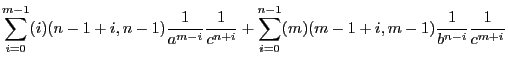 |
|||
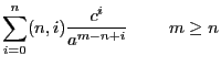 |
|||
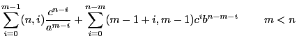 |
Actually the ratio statement is a leftover from the Schoonschip inheritance. For most simple partial fractioning one could use
   repeat id 1/[x+a]/[x+b] = (1/[x+a]-1/[x+b])/[b-a];
   repeat id [x+a]/[x+b] = 1-[b-a]/[x+b];
   repeat id [x+b]/[x+a] = 1+[b-a]/[x+a];
or similar constructions. This does not give the speed of the binomials, but it does make the program more readable and it is much more flexible.
| Type | Executable statement |
| Syntax | rc[yclesymmetrize] {<name of function/tensor>
[<argument specifications>];} |
| See also | symmetrize (7.141), cyclesymmetrize (7.28), antisymmetrize (7.4) |
The argument specifications are explained in the section on the symmetrize statement (see 7.141).
The action of this statement is to
reverse-cycle-symmetrize
the (specified) arguments of the functions
that are mentioned. This means that the arguments are brought to `natural
order' in the notation of FORM by trying cyclic and reverse cyclic
permutations of the arguments or groups of arguments.
The `natural order' may depend on the order of declaration of the
variables.
| Type | Executable statement |
| Syntax | r[edefine] <preprocessor variable> "<string>"; |
| See also | preprocessor variables in the chapter on the preprocessor (3) |
This statement can be used to change the contents of preprocessor variables. The new contents can be used after the current module has finished execution and the preprocessor becomes active again for further translation and compilation. This termwise adaptation of the value of a preprocessor variable can be very useful in setting up multi module loops until a certain condition is not met any longer. Example:
   #do i = 1,1
      statements;
      if ( condition ) redefine i "0";
      .sort
   #enddo
As long as there is a term that fulfils the condition the loop
will continue. This defines effectively a while loop (see
7.160) over various modules. Note that the .sort
instruction is essential. Note also that a construction like
if ( count(x,1) > 3 ) redefine i "`i'+1";is probably not going to do what the user intends. It is not going to count terms with more than three powers of x. The preprocessor will insert the compile time value of the preprocessor variable i. If this is 0, then each time a term has more than three powers of x, i will get the string value
0+1. If one would like to do such counting, one should use a
dollar variable (see 6).
| Type | Executable statement |
| Syntax | removespectator <spectator;>; |
See chapter20 on spectators.
| Type | Executable statement |
| Syntax | renumber <number>; |
| See also | sum (7.138) |
Renumbers the dummy
indices. Dummy indices are indices of the type
N1_?. Normally FORM tries to renumber these indices to make the
internal representation of a term `minimal'. It does not try exhaustively
though. Especially interference with symmetric or antisymmetric functions
is far from perfect. This is due to considerations of economy. With the
renumber statement the user can force FORM to do better. The allowable
options are:
| 0 |
| All exchanges of one pair of dummy indices are tried until all pair exchanges yield no improvements. This is the default if no option is specified. |
| 1 |
| If there are N sets of dummy indices all N! permutations are tried. This can be very costly when a large number of indices is involved. Use with care! |
| Type | Executable statement |
| Syntax | repeat; |
| repeat <executable statement> | |
| See also | endrepeat (7.48), while (7.160) |
The repeat statement starts a
repeat environment. It is terminated with an
endrepeat statement (see 7.48). The
repeat statement and its matching endrepeat statement should be inside the
same module.
The statements inside the repeat environment should all be executable statements (or print statements) and if any of the executable statements inside the environment has changed the current term, the action of the endrepeat statement will be to bring control back to the beginning of the environment. In that sense the repeat/endrepeat combination acts as
   do
      executable statements
   while any action due to any of the statements
The second form of the statement is a shorthand notation:
   repeat;
      single statement;
   endrepeat;
is equivalent to
repeat single statement;Particular attention should be given to avoid infinite loops as in
repeat id a = a+1;A more complicated infinite loop is
   repeat;
      id  S(x1?)*R(x2?) = T(x1,x2,x2-x1);
      id  T(x1?,x2?,x3?pos_) = T(x1,x2-2,x3-1)*X(x2);
      id  T(x1?,x2?,x3?) = S(x1)*R(x2);
   endrepeat;
If the current term is S(2)*R(2), the statements in the loop do not change
it in the end. Yet the program goes into an infinite loop, because the
first id statement will change the term (action) and the third statement
will change it back. FORM does not check that the term is the same
again. Hence there is action inside the repeat environment and hence the
statements will be executed again. This kind of hidden action is a major
source of premature
terminations of FORM programs.
Repeat environments can be nested with all other
environments (and of course also with other repeat/endrepeat combinations).
| Type | Executable statement |
| Syntax | replaceloop <parameters>; |
| See also | the findloop option of the if statement (7.71) |
This statement causes the substitution of index loops. An index loop is a sequence of contracted indices in which the indices are arguments of various instances of the same function and each contracted index occurs once in one instance of the function and once in another instance of the function. Such a contraction defines a connection and if a number of such connections between occurrences of the function form a loop this structure is a candidate for replacement. Examples of such loops are:
    f(i1,i2,j1)*f(i2,i1,j2)
    f(i1,i2,j1)*f(i2,i3,j2)*f(i1,i3,j3)
    f(i1,k1,i2,j1)*f(k2,i2,i3,j2)*f(i1,k3,i3,j3)
The first term has a loop of two functions or vertices and
the other two terms each define a loop of three vertices. The parameters
are:
| The name of the function that defines the `vertices'. This must always be the first parameter. |
| arguments=number |
| Only occurrences of the vertex function with the specified number of arguments will be considered. The specification of this parameter is mandatory. |
| loopsize=number |
| Only a loop with this number of vertices will be considered. |
| loopsize=all |
| All loop sizes will be considered and the smallest loop is substituted. |
| loopsize |
| Only loops with fewer vertices than `number' will be considered and the smallest looop will be substituted. |
| outfun= |
| Name of an output function in which the remaining arguments of all the vertex functions will be given. This parameter is mandatory. |
| include- |
| Name of a summable index that must be one of the links in the loop. This parameter is optional. |
The loopsize parameter is mandatory. Hence one of its options must be specified. The order of the parameters is not important. The only important thing is that the name of the vertex function must be first. The names of the keywords may be abbreviated as in
ReplaceLoop f,a=3,l=all,o=ff,i=i2;
although this does not improve the readability of the program. Hence a more
readable abbreviated version might be
ReplaceLoop f,arg=3,loop=all,out=ff,inc=i2;
The action of the statement is to remove the vertex functions that constitute the loop and replace them by the output function. This outfun will have the arguments of all the vertex functions minus the contracted indices that define the loop. The order of the arguments is the order in which they are encountered when following the loop. The order of the arguments in the outfun depends however on the order in which FORM encounters the vertices. Hence the outfun will often be cyclesymmetric (see 7.62 and 7.28). If FORM has to exchange indices to make a `proper loop' (i.e. giving relevance to the first index as if it is something incoming and the second index as if it is something outgoing) and if the vertex function is antisymmetric, each exchange will result in a minus sign. Examples:
    Functions f(antisymmetric),ff(cyclesymmetric);
    Indices i1,...,i8;
    Local F = f(i1,i4,i2)*f(i5,i2,i3)*f(i3,i1,i6)*f(i4,i7,i8);
    ReplaceLoop f,arg=3,loop=3,out=ff;
would result in
-f(i4,i7,i8)*ff(i4,i5,i6)
and
    Functions f(antisymmetric),ff(cyclesymmetric);
    Indices i1,...,i9;
    Local F = f(i1,i4,i2)*f(i5,i2,i3)*f(i3,i1,i6)*f(i4,i7,i8)
            *f(i6,i7,i8);
    ReplaceLoop f,arg=3,loop=all,out=ff;
would give
-f(i1,i4,i2)*f(i5,i2,i3)*f(i3,i1,i6)*ff(i4,i6)
because the smallest loop will be taken. A number of examples can be found
in the package `color' for group
theory invariants that is part of the FORM
distribution.
A related object is the findloop option of the
if statement (see 7.71). This option just probes
whether a loop is present but makes no replacements.
| Type | Declaration statement |
| Syntax | sa[ve] <filename> [<names of global expressions>]; |
| See also | load (7.83) |
Saves the contents of the store file (all global expressions that were stored in .store instructions) to a file with the indicated name. If a list of expressions is provided only those expressions are saved and the others are ignored.
Together with the load statement (see 7.83) the save statement provides a mechanism to transfer data in internal notation from one program to another. It is the preferred method to keep results of a lengthy job for further analysis without the need for the long initial running time.
In order to avoid confusion .sav is the
preferred extension of saved files.
| Type | Executable statement |
| Syntax | select <list of sets> <pattern> = <expression>; |
| See also | identify (7.68) |
This statement is identical to the select option of the id statement (see 7.68). Hence
select ....is just a shorthand notation for
id select ....
| Type | Declaration statement |
| Syntax | set <set to be declared>[(option)]:<element> [<more elements>]; |
Declares a single set and specifies its elements. Sets have a type of variables connected to them. There can be sets of symbols, sets of functions, sets of vectors, sets of indices and sets of numbers. For the purpose of sets tensors and tables count as functions.
There can also be mixed sets of indices and numbers. When a number could be either a fixed index or just a number FORM will keep the type of the set unfixed. This can change either when the next element is a symbolic index or a number that cannot be a fixed index (like a negative number). If the status does not get resolved the set can be used in the wildcarding of both symbols and indices. Normally sets of numbers can be used only in the wildcarding of symbols.
Currently the only option is the ordered set, indicated by
Set name(ordered):x4,x3,x1,x6,x2;
which would be stored as x1,x2,x3,x4,x6 if that would be the order of
declaration.
| Type | Executable statement |
| Syntax | setexitflag; |
| See also | exit (7.52) |
Causes termination of the
program after execution of the current module has
finished.
| Type | Executable statement |
| Syntax | shuffle,functionname; |
| shuffle,once,functionname; | |
| See also | stuffle (7.137) |
| merge (7.87) |
This statement is exactly the same as the merge statement. It takes two occurrences of the mentioned function and outputs terms, each with one function in which the two argument lists have been merged in all different ways, keeping the relative ordering of the two lists preserved. It is the opposite of the distrib_ function (see 8.12). Hence
   Local F = f(a,b)*f(c,d);
   shuffle,f;
will result in
+f(a,b,c,d)+f(a,c,b,d)+f(a,c,d,b)+f(c,a,b,d)+f(c,a,d,b)+f(c,d,a,b)
One can also obtain the same result with the statements
   Multiply,ff;
   repeat id f(x1?,?a)*f(x2?,?b)*ff(?c) =
            +f(?a)*f(x2,?b)*ff(?c,x1)
            +f(x1,?a)*f(?b)*ff(?c,x2);
   id f(?a)*f(?b)*ff(?c) = f(?c,?a,?b);
but the advantage of the shuffle statement is that is also does a certain
amount of combinatorics when there are identical arguments. Unfortunately
the combinatorics doesn't extend over groups of arguments that are
identical as in
    CF  f;
    L   F = f(0,1,0,1,0,1)*f(0,1,0,1,0,1);
    Shuffle,f;
    .end

Time =       0.00 sec    Generated terms =        141
               F         Terms in output =         32
                         Bytes used      =        892
It does get the combinatorics between two zeroes or two ones, but it cannot
handle the groups. The explicit method above however doesn't do any
combinatorics and generates 924 terms.
One of the applications of this statement is in the field of harmonic sums, harmonic polylogarithms and multiple zeta values. Its twin brother is the stuffle statement (see 7.137).
When the option once is mentioned, only one pair will be contracted this
way. Without this option all occurrences of the function inside a term will
be treated till there are only terms with a single occurrence of the
function.
| Type | Specification statement |
| Syntax | skip; |
| skip <list of expressions>; | |
| See also | nskip (7.100) |
In the first variety this statement marks all
active expressions that are in existence at the moment this
statement is compiled, to be skipped. In the second variety this is done
only to the active expressions that are specified. If an expression is
skipped in a given module, the statements in the module have no effect on
it. Also it will not be sorted again at the end of the module.
This means that any bracket information (see
7.11) in the expression remains the way it was. Consult also
the nskip statement in 7.100.
Skipped expressions can be used in the expressions in the r.h.s.
of id statements (see 7.68) or
multiply statements (see 7.92), etc.
| Type | Executable statement |
| Syntax | sort; |
| See also | term (7.145), endterm (7.50) |
Statement to be used inside the term
environment (see 7.145 and
7.50). It forces a sort in the same way as a
.sort instruction forces a sort for entire expressions.
| Type | Executable statement |
| Syntax | splitarg options {<name of function/set>
[<argument specifications>]}; |
| See also | splitfirstarg (7.135), splitlastarg (7.136), factarg (7.54) |
Takes the indicated argument of a function and if such an argument is a subexpression that consists on more than one term, all terms become single arguments of the function as in
f(a+b-5*c*d) --> f(a,b,-5*c*d)The way arguments are indicated is rather similar to the way this is done in the argument statement (see 7.9). One can however indicate only a single group of functions in one statement. Additionally there are other options. All options are in the order that they should be specified:
| (term) |
| Only terms that are a numerical multiple of the given term are split off. The terms that are split off will trail the remainder. |
| ((term)) |
| Only terms that contain the given term will be split off. The terms that are split off will trail the remainder. |
The statement is terminated with a sequence of functions or sets of functions. The splitting action will apply only to the specified functions or to members of the set(s). If no functions or sets of functions are specified all functions will be treated, including the built in functions.
The argument specifications consist of a list of numbers,
indicating the arguments that should be treated. If no arguments are
specified, all arguments will be treated.
| Type | Executable statement |
| Syntax | splitfirstarg {<name of function/set>
[<argument specifications>]}; |
| See also | splitarg (7.134), splitlastarg (7.136) |
A little bit like the SplitArg statement (see 7.134). Splits the given argument(s) into its first term and a remainder. Then replaces the argument by the remainder, followed by the first term.
The statement is terminated with a sequence of functions or sets of functions. The splitting action will apply only to the specified functions or to members of the set(s). If no functions or sets of functions are specified all functions will be treated, including the built in functions.
The argument specifications consist of a list of numbers,
indicating the arguments that should be treated. If no arguments are
specified all arguments will be treated.
| Type | Executable statement |
| Syntax | splitlastarg {<name of function/set>
[<argument specifications>]}; |
| See also | splitarg (7.134), splitfirstarg (7.135) |
A little bit like the SplitArg statement (see 7.134). Splits the given argument(s) into its last term and a remainder. Then replaces the argument by the remainder, followed by the last term.
The statement is terminated with a sequence of functions or sets of functions. The splitting action will apply only to the specified functions or to members of the set(s). If no functions or sets of functions are specified all functions will be treated, including the built in functions.
The argument specifications consist of a list of numbers,
indicating the arguments that should be treated. If no arguments are
specified all arguments will be treated.
| Type | Executable statement |
| Syntax | stuffle,functionname+; |
| stuffle,functionname-; | |
| stuffle,once,functionname+; | |
| stuffle,once,functionname-; | |
| See also | shuffle (7.131) |
This statement
takes two occurrences of the mentioned function and outputs
terms, each with one function in which the two argument lists have been
merged according to the rules for nested sums. The plus and minus signs
refer to ones favorite definition for nested sums. In the case of the plus
sign, the definition is
 |
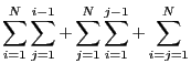 |
(7.4) |
|
 |
(7.5) |
    CF  S,R;
    Symbols N,n;
    L   F = S(R(1,-3),N)*S(R(-5,1),N);
    id  S(R(?a),n?)*S(R(?b),n?) = S(?a)*S(?b)*R(n);
    Stuffle,S-;
    id  S(?a)*R(n?) = S(R(?a),n);
    Print +s;
    .end

Time =       0.00 sec    Generated terms =         12
               F         Terms in output =         12
                         Bytes used      =        462

   F =
       + S(R(-6,-4),N)
       - S(R(-6,-3,1),N)
       - S(R(-6,1,-3),N)
       - S(R(-5,1,-4),N)
       + S(R(-5,1,-3,1),N)
       + 2*S(R(-5,1,1,-3),N)
       - S(R(-5,2,-3),N)
       - S(R(1,-5,-4),N)
       + S(R(1,-5,-3,1),N)
       + S(R(1,-5,1,-3),N)
       + S(R(1,-3,-5,1),N)
       - S(R(1,8,1),N)
      ;
The above program is equivalent to the basis procedure in the summer
library. As with the shuffle statement (see
7.131) a certain amount of combinatorics has been built in.
When the option once is mentioned, only one pair will be contracted this way. Without this option all occurrences of the function inside a term will be treated till there are only terms with a single occurrence of the function.
The stuffle command takes also the effect of roots of
unity 7.140 into account in the same way
that the signs of alternating sums are taken into account. This means that
the sum indices don't have to be integers, but could be multiples of a
single symbol that has been declared to be a root of
unity 7.140.
| Type | Executable statement |
| Syntax | sum <list of indices>; |
| See also | renumber (7.124) |
The given indices will be summed over. There are two
varieties. In the first the index is followed by a sequence of nonnegative
short integers. In that case the summation means that for each of the
integers a new instance of the term is created in which the index is
replaced by that integer. In the second variety the index is either the
last object in the statement or followed by another index. In that case the
index is replaced by an internal dummy
index of the type N1_? (or with another number
instead of the 1). Such indices have the current
default dimension and can
be renamed at will by FORM to bring terms into standard notation. For
example:
f(N2_?,N1_?)*g(N2_?,N1_?)will be changed into
f(N1_?,N2_?)*g(N1_?,N2_?).The user can use these dummy indices in the left hand side of id statements.
| Type | Executable statement |
| Syntax | switch,$-variable; |
| See also | case (7.13), break (7.12), default(7.30), endswitch (7.49). |
The argument of the switch statement should be a dollar variable
which evaluates into an integer that first inside a FORM word.
On a 64-bit processor this would be an integer in the range ![]() to
to
![]() . The switch statement should be paired with an endswitch
statement. Between the two there will be a number of cases, each marked by
an integer. If the value of the dollar variable corresponds to the value of
one of these cases, execution will continue with the first statement after
the corresponding case statement. Example:
. The switch statement should be paired with an endswitch
statement. Between the two there will be a number of cases, each marked by
an integer. If the value of the dollar variable corresponds to the value of
one of these cases, execution will continue with the first statement after
the corresponding case statement. Example:
    id  f(x?$x) = f(x);
    switch $x;
      case -1;
        some statements
      break;
      case 3;
        more statements
      break;
      case 4;
      case 5;
        and a few more
      break;
      default;
        and the default action
      break;
    endswitch;
In principle the action is the same as in any computer language that has a
switch construction, including the fall-through between case 4 and case 5.
Whether the selection of the cases goes by binary search in a sorted list
or by jumptable is determined by the endswitch statement.
| Type | Declaration statement |
| Syntax | s[ymbols] <list of symbols to be declared>; |
Declares one or more symbols. Each symbol can be followed by a number of options. These are (assuming that x is the symbol to be declared):
| x#r |
| The symbol is real. This is the default. |
| x#c |
| The symbol is complex. This means that two spaces are reserved for this symbol, one for x and one for x#(the complex conjugate). |
| x#i |
| The symbol is imaginary. |
| x#=number |
| The symbol is a number-th root of unity This means that the number-th power of the symbol will be replaced by one and half this power (if even) by -1. Negative powers will be replaced by corresponding positive powers. |
| x(:5) |
| The symbol has the maximum power 5. This means that |
| x(-3:) |
| The symbol has the minimum power -3. This means that
|
| x(-3:5) |
| The combination of a maximum and a minimum power restriction (see above). |
Complexity properties and power restrictions can be combined. In
that case the complexity properties come first and then the power
restrictions.
| Type | Executable statement |
| Syntax | symm[etrize] {<name of function/tensor>
[<argument specifications>];} |
| See also | antisymmetrize (7.4), cyclesymmetrize (7.28), rcyclesymmetrize (7.121) |
The arguments consist of the name of a function
(or a tensor), possibly followed by some specifications. Hence we have the
following varieties:
| <name> |
| The function is symmetrized in all its arguments. |
| <name><numbers> |
| The function is symmetrized in the arguments that are mentioned. If there are fewer arguments than the highest number mentioned in the list or arguments, no symmetrization will take place. |
| <name>:<number> |
| Only functions with the specified number of arguments will be considered. Note: the number should follow the colon directly without intermediate space or comma. |
| <name>:<number><numbers> |
| If there is a number immediately following the colon, only functions with exactly that number of arguments will be considered. If the list of arguments contains numbers greater than this number, they will be ignored. If no number follows the colon directly, this indicates that symmetrization will take place, no matter the number of arguments of the function. If the list of arguments has numbers greater than the number of arguments of the function, these numbers will be ignored. |
| <name>
<(groups of numbers)> |
| The groups are specified as lists of numbers of arguments between parenthesis. All groups must have the same number of arguments or there will be a compile error. The groups are symmetrized as groups. The arguments do not have to be adjacent. Neither do they have to be ordered. The symmetrization takes place in a way that the first elements of the groups are most significant, etc. If any argument number is greater than the number of arguments of the function, no symmetrization will take place. |
| <name>:<number>
<(groups of numbers)> |
| The groups are specified as lists of numbers of arguments between parenthesis. All groups must have the same number of arguments or there will be a compile error. The groups are symmetrized as groups. The arguments do not have to be adjacent. Neither do they have to be ordered. The symmetrization takes place in a way that the first elements of the groups are most significant, etc. If no number follows the colon directly symmetrization takes place no matter the number of arguments of the function. Groups that contain a number that is greater than the number of arguments of the function will be ignored. If a number follows the colon directly, only functions with that number of arguments will be symmetrized. Again, groups that contain a number that is greater than the number of arguments of the function will be ignored. |
The action of this statement is to symmetrize the
(specified) arguments of the functions that are mentioned. This means that
the arguments are brought to `natural order' in the notation of FORM by
trying permutations of the arguments or groups of
arguments. The `natural order' may depend on the order of declaration of
the variables.
Examples:
   Symmetrize Fun;
   Symmetrize Fun 1,2,4;
   Symmetrize Fun:5;
   Symmetrize Fun: 1,2,4;
   Symmetrize Fun:5 1,2,4;
   Symmetrize Fun (1,6),(7,3),(5,2);
   Symmetrize Fun:8 (1,6),(7,3),(5,2);
   Symmetrize Fun: (1,6),(7,3),(5,2);
| Type | Declaration statement |
| Syntax | table <options> <table to be declared>; |
| See also | functions (7.62), ctable (7.26), ntable (7.101), fill (7.57) |
The statement declares a single table. A table is a
very special instance of a function. Hence it can be either
commuting or noncommuting. The table
statement declares its function to be commuting. A noncommuting table is
declared with the ntable statement (see 7.101).
A table has a number of table indices (in the case of
zero indices the table has to be sparse) and after that it can have a
number of regular function arguments with or without wildcarding. The table
indices can come in two varieties: matrix like or
sparse. In the case of a matrix like table, for each of the indices a range has to be specified. FORM then
reserves a location for each of the potential elements. For a sparse
table one only specifies the number of indices. Sparse
tables take less space, but they require more time searching whether an
element has been defined. For a matrix like table FORM can look directly
whether an element has been defined. Hence one has a tradeoff between space
and speed. A zero-dimensional (sparse) table has of course only a single
element.
Table elements are defined with the fill statement (see
7.57). Fill statements for table elements cannot be used before
the table has been declared with a table or ntable statement.
When FORM encounters an unsubstituted table it will look for its indices. Then it can check whether the table element has been defined. If not, it can either complain (when the `strict' option is used) or continue without substitution. Note that an unsubstituted table element is a rather expensive object as FORM will frequently check whether it can be substituted (new elements can be defined in a variety of ways....). If the indices match a defined table element, FORM will check whether the remaining arguments of the table will match the function-type arguments given in the table declaration in the same way regular function arguments are matched. Hence these arguments can contain wildcards and even argument field wildcards. If a match occurs, the table is replaced immediately.
The options are
| check |
| A check is executed on table boundaries. An element that is outside the table boundaries (regular matrix type tables only) will cause an error message and execution will be halted. |
| relax |
| Normally all elements of a table should be defined during execution and an undefined element will give an error message. The relax option switches this off and undefined elements will remain as if they are regular functions. |
| sparse |
| The table is considered to be sparse. In the case of a sparse table only the number of indices should be specified. Ranges are not relevant. Each table element is stored separately. Searching for table elements is done via a balanced tree. This takes of course more time than the matrix type search with is just by indexing. A matrix like table is the default. |
| strict |
| If this option is specified all table elements that are encountered during execution should be defined. An undefined table element will result in an error and execution is halted. Additionally all table elements should be properly defined at the end of the module in which the table has been defined. |
| zerofill |
| Any undefined table element is considered to be zero. |
| onefill |
| Any undefined table element is considered to be one. |
The defaults are that the table is matrix like and table elements
that cannot be substituted will result in an error.
Ranges for indices in matrix like tables are indicated with a colon as in
   Symbol x;
   Table t1(1:3,-2:4);
   Table t2(0:3,0:3,x?);
   Table sparse,t3(4);
The table
t1 is two dimensional and has 21 elements. The table
t2 is also two dimensional and has 16 elements. In addition there is
an extra argument which can be anything that a wildcard symbol will match.
The table t3 is a sparse table with 4 indices.
If the computer on which FORM runs is a 32 bit
computer no table can have more than
![]() elements. On a
64 bit computer the limit is
elements. On a
64 bit computer the limit is ![]() , but one should take
into account that each element declared causes some overhead.
, but one should take
into account that each element declared causes some overhead.
If the wildcarding in the declaration of a table involves the definition of a dollar variable (this is allowed! See 6) parallel execution of the entire remainder of the FORM program is switched off. This is of course only relevant for parallel versions of FORM. But if at all possible one should try to find better solutions than this use of dollar variables, allowing future parallel processing of the program.
In some cases tables are built up slowly during the execution of
a program and used incrementally. This means that more and more CPU memory
is needed. Eventually this can cause a crash by lack of memory. In the case
that the earlier elements of the table aren't needed anymore, one could use
the ClearTable 7.18 statement.
This statement is explained in the chapter on
tablebases (12).
| Type | Declaration statement |
| Syntax | t[ensors] <list of tensors to be declared>; |
| See also | functions (7.62), ctensors (7.27), ntensors (7.102) |
A tensor is a special function that can have only indices for its arguments. If an index a contracted with the index of a vector Schoonschip notation is used. This means that the vector is written as a pseudo argument of the tensor. It should always be realized that in that case in principle the actual argument is a dummy index. Tensors come in two varieties: commuting and noncommuting. The tensor statement declares a tensor to be commuting. In order to declare a tensor to be noncommuting one should use the ntensor statement (see 7.102).
The options that exist for properties of tensors are the same as
those for functions (see 7.62).
| Type | Executable statement |
| Syntax | term; |
| See also | endterm (7.50), sort (7.133) |
Begins the term environment.
This environment is terminated with the endterm statement
(see 7.50). The action is that temporarily the current term
is seen as a little expression by itself. The statements inside the
environment are applied to it and one can even sort the results with the
sort statement (see 7.133) which should not be
confused with the .sort instruction that terminates a module.
Inside the term environment one can have only executable statements and
possibly term-wise print statements (see 7.113). When the end
of the term environment is reached, the results are sorted (as would be
done with an expression at the end of a module) and execution continues
with the resulting terms. This environment can be nested.
| Type | Executable statement |
| Syntax | testuse ["<tablename(s)>"]; |
| See also | tablebases (12), testuse (12.10) |
This statement is explained in the chapter on
tablebases.
| Type | Declaration |
| Syntax | ThreadBucketSize,number; |
| See also | the section on TFORM(18.1) |
This statement is only active in
TFORM. In all other versions of FORM it is ignored. It sets
the size of the buckets that the master thread
prepares for treatment by the workers. Bigger buckets means less overhead
in signals, but when the buckets are too big the workers may have to wait
too long before getting tasks. The best bucket size is usually between 100
and 1000, although this depends very much on the problem. The default value
is currently 500. For more ways to set this variable one should consult the
section on TFORM (18.1). To find out what its value is, use the
`ON,setup;' statement (7.107 and 17).
| Type | Executable statement |
| Syntax | topolynomial[,OnlyFunctions[,<list of functions>]]; |
| See also | factarg (7.54), FromPolynomial (7.61), ArgToExtraSymbol (7.8) |
| and ExtraSymbols (7.53, 2.11). |
Starting with version 4.0 of FORM some built in operations or statements can only deal with symbols and numbers. Examples of this are factorization (7.54) and output simplification (still to be implemented). The ToPolynomial statement takes each term, looks for objects that are not symbols to positive powers and replaces them by symbols. If the object has been encountered before, the same symbol will be used, otherwise a new symbol will be defined. The object represented by the `extra symbol' is stored internally and can be printed if needed with the %X option in the #write instruction (3.64). Note that negative powers of symbols will also be replaced.
In some cases one would like to do this only for a subset of objects. It is
possible to do this only for functions, using the OnlyFunctions option. If
no functions are specified, all functions will be replaced by extra
symbols. If a list of functions is specified, only those functions will be
replaced.
| Type | Executable statement |
| Syntax | tospectator <spectator;>; |
See chapter20 on spectators.
| Type | Executable statement |
| Syntax | totensor [nosquare] [functions] [!<vector or set>] <vector> <tensor>; |
| totensor [nosquare] [functions] [!<vector or set>] <tensor> <vector>; | |
| See also | tovector (7.151) |
Looks for multiple occurrences of the given
vector, either inside dotproducts, contracted with a tensor, as argument of
a function or as a loose vector with an index. In all occurrences in
which the vector has been contracted a dummy index is introduced to make
the contraction apparent. Then all these vectors with their indices are
replaced by the specified tensor with all the indices of these vectors. To
make this clearer:
p.p1^2*f(p,p1)*p(mu)*tt(p1,p,p2,p)gives after
totensor p,t;
f(N1_?,p1)*tt(p1,N2_?,p2,N3_?)*t(p1,p1,mu,N1_?,N2_?,N3_?)
The options are
| nosquare |
| Dotproducts with twice the specified vector (square of the vector) are not taken into account. |
| functions |
| Vectors that are arguments of regular functions will also be considered. By default this is not done. |
| !vector |
| Dotproducts involving the specified vector are not treated. |
| !set |
| The set should be a set of vectors. All dotproducts involving a vector of the set are not treated. |
| Type | Executable statement |
| Syntax | tovector <tensor> <vector>; |
| tovector <vector> <tensor>; | |
| See also | totensor (7.150) |
The opposite of the totensor
statement. The tensor is replaced by a product of the given vectors, each
with one of the indices of the tensor as in:
| Type | Executable statement |
| Syntax | trace4 [<options>] <index>; |
| See also | tracen (7.153), chisholm (7.17), unittrace (7.158) |
| and the chapter on gamma algebra (14) |
Takes the trace of the gamma
matrices with the given trace line
index. It assumes that the matrices are
defined in four dimensions, hence it uses some relations that are only
valid in four dimensions. For details about these relations and other
methods used, consult chapter 14 on gamma matrices. The
options are:
| contract |
| Try to use the Chisholm identity to eliminate this trace and contract it with other gamma matrices. See also 7.17. This is the default. |
| nocontract |
| Do not use the Chisholm identity to eliminate this trace and contract it with other gamma matrices. See also 7.17. |
| nosymmetrize |
| When using the Chisholm identity to eliminate this trace and contract it with other gamma matrices, do not do it in the symmetric fashion, but use the first contraction encountered. See also 7.17. |
| notrick |
| The final stage of trace taking, when all indices are different
and there are no contractions with identical vectors, as well as no
|
| symmetrize |
| When using the Chisholm identity to eliminate this trace and contract it with other gamma matrices, try to do it in the symmetric fashion. See also 7.17. |
| trick |
| The final stage of trace taking, when all indices are different
and there are no contractions with identical vectors is done using the
4-dimensional relation
This gives a shorter result for long traces. It is the default. |
| Type | Executable statement |
| Syntax | tracen <index>; |
| See also | trace4 (7.152), chisholm (7.17), unittrace (7.158) |
| and the chapter on gamma algebra (14) |
Takes the trace of the gamma
matrices with the spin line indicated by the index. It is
assumed that the trace is over a symbolic number of dimensions. Hence no
special 4-dimensional tricks are used. The presence of ![]() ,
,
![]() or
or ![]() is not tolerated. When indices are contracted
FORM will try to use the special symbol for the dimension
is not tolerated. When indices are contracted
FORM will try to use the special symbol for the dimension![]() if it has
been defined in the declaration of the index (see 7.74. This
results in relatively compact expressions. For more details on the
algorithm used, see chapter 14 on gamma matrices.
if it has
been defined in the declaration of the index (see 7.74. This
results in relatively compact expressions. For more details on the
algorithm used, see chapter 14 on gamma matrices.
| Type | Executable statement |
| Syntax | transform,function(s),<one or more transformations>; |
Statement to manipulation function arguments and fields of arguments. Allows speedy transformations without the need of multiple statements or repeat loops.
The function(s) is/are indicated as individual, comma or blank space separated, functions or sets of functions.
If there is more than one transformation, the transformations are separated by comma's (or blanks, unless the blank space would not induce a comma).
Each transformation consists of its keyword, indicating its type, followed by a range of arguments that is enclosed by parentheses. After that specific information may follow. The range is as in
	(1,4)
	(3,last)
	(last-6,last-2)
hence two indicators, separated by a comma. If the first number is bigger than the second the arguments will be processed in reverse order whenever this is relevant. In the descriptions below we will indicate the range by (r1,r2). The numbers in the above examples may be also dollar variables, provided they evaluate into numbers at the time of execution. Hence
	($x,$y)
	($x,last)
	(last-$x,last-2)
are potentially legal ranges. One may not use
$x+2 or other
expressions that still need evaluation.
The transformations that are allowed currently are:
| replace |
| replace(r1,r2)=(from1,to1,from2,to2,...,fromn,ton) in
which the from-to pairs are as in the replace_ function. Here however
there are more options than in the replace_ function as we can specify
(small) numbers as well as in
replace(1,last)=(0,1,1,0) which would replace arguments that are zero by one and arguments that are one by zero. Generic arguments are indicated by the new variables xarg_, iarg_, parg_ and farg_ as in replace(1,last)=(xarg_,2xarg_+1,p) which would replace f(2,a) by f(5, 2a+1,p) if a is a symbol and p a vector. To catch p one would need to use parg_. |
| encode |
| encode(r1,r2):base=number will interprete the arguments as the digits in a base 2 number system, compute the complete number and replace the arguments by a single argument that is that number. The number must fit inside a single FORM word and so must each of the original arguments. They should actually be smaller than the number of the base. |
| decode |
| decode(r1,r2):base=number will do the opposite of encode. It will take a single argument (the smallest of the two given) and expand it into digits in a number system given by the base. It will create the specified number of digits and replace the original number by the given number of arguments representing these digits. If r2 is less than r1 the digits will be in reverse order. |
| tosumnotation |
| tosumnotation(r1,r2) or implode(r1,r2) realizes an encoding in which zeroes are absorbed as extra values in the first nonzero argument that is following. This is used when dealing with harmonic sums and harmonic polylogarithms. An example is that (0,0,1,0,a,0,0,0,-1) (which is in integral notation) goes into (3,2*a,-4) (which is in sum notation). Currently only a single symbol is allowed and the numbers should be (small) integers because otherwise the reverse operation (explode) would generate too many arguments. Instead of ``tosumnotation'' one may also use the word ``implode'' in accordance with the argimplode statement. |
| tointegralnotation |
| tointegralnotation(r1,r2) or explode(r1,r2) undoes what
implode might have done. Hence each integer with an absolute value |
| permute |
| permute(1,3,5)(2,6) will permute the arguments
according to the cycles indicated. The cycles are executed in order and may
overlap. Their number is not restricted. In the above example
f(a1,a2,a3,a4,a5,a6,a7) |
| reverse |
| reverse(r1,r2) reverses the order of the arguments in specified range. |
| dedup |
| dedup(r1,r2) removes duplicates from the arguments in the range, keeping the first. |
| cycle |
| cycle(r1,r2)=+/-number will perform a cyclic permutation of the indicated range of arguments. If the number is preceeded by a - the cycling is to the left. If there is a plus sign the cycling is to the right. Note that either the plus or the minus sign is mandatory. The number following the +/- sign is also allowed to be a dollar variable provided it evaluates to a legal number during execution. |
| islyndon |
| islyndon(r1,r2)=(yes,no) will test whether the indicated
range of arguments forms a Lyndon word according to the
ordering of arguments in FORM. The yes and no arguments are what the main
term will be multiplied by when the range forms a Lyndon word or does not
respectively. Because the definition of a Lyndon word is the unique minimal
cyclic permutation of the arguments, and because often we may need the
unique maximal cyclic permutation there are varieties: for the minimum one
may also use islyndon |
| tolyndon |
| tolyndon(r1,r2)=(yes,no) will permute the given range in
a cyclic manner till it is (if possible) a Lyndon word
according to the ordering of arguments in FORM. The yes and no arguments
are what the main term will be multiplied by when afterwards the range
forms a Lyndon word or does not respectively. Because the definition of a
Lyndon word is the unique minimal cyclic permutation of the arguments, and
because often we may need the unique maximal cyclic permutation there are
varieties: for the minimum one may also use tolyndon |
| addargs |
| addargs(r1,r2) replaces the indicated range of arguments by their sum. This is effectively the inverse of the SplitArg statement. |
| mulargs |
| mulargs(r1,r2) replaces the indicated range of arguments by their product. This is effectively the inverse of the FactArg statement. |
| dropargs |
| dropargs(r1,r2) removes the indicated range of arguments. |
| selectargs |
| selectargs(r1,r2) removes all arguments with the exception of the indicated range of arguments. |
Some Examples. Assume that we have some Multiple Zeta Values (see the papers on harmonic sums, harmonic polylogarithms and the MZV data mine) in the sum notation, but for calculational reason we want to use a binary encoding (as used in the MZV programs). We could have
    Symbol x,x1,x2;
    CF  H,H1;
    Off Statistics;
    L   F = H(3,4,2,6,1,1,1,2);
    repeat id H(?a,x?!{0,1},?b) = H(?a,0,x-1,?b);
    Print;
    .sort

   F =
      H(0,0,1,0,0,0,1,0,1,0,0,0,0,0,1,1,1,1,0,1);

    Multiply H1;
    repeat id H(x?,?a)*H1(?b) = H(?a)*H1(?b,1-x);
    id  H1(?a)*H = H(?a);
    Print;
    .sort

   F =
      H(1,1,0,1,1,1,0,1,0,1,1,1,1,1,0,0,0,0,1,0);

    repeat id H(x1?,x2?,?a) = H(2*x1+x2,?a);
    Print;
    .end

   F =
      H(907202);
The new version of the same program would be
    Symbol x,x1,x2;
    CF  H,H1;
    Off Statistics;
    L   F = H(3,4,2,6,1,1,1,2);
    Transform,H,explode(1,last),
                replace(1,last)=(0,1,1,0),
                encode(1,last):base=2;
    Print;
    .end

   F =
      H(907202);
It should be clear that this is simpler and faster. On a 64-bits computer
it is faster by more than a factor 100.
| Type | Executable statement |
| Syntax | tryreplace {<name> <replacement>}; |
| See also | the replace_ function (8.58) |
The list of potential replacements should be
similar to the arguments of the replace_
function (see 8.58). FORM will
make a copy of the current term, try the replacement and if the replacement
results in a term which, by the internal ordering of FORM, comes before
the current term, the current term is replaced by the new variety.
| Type | Output control statement |
| Syntax | unfactorize {<name of expression(s)>}; |
| See also | the chapter on polynomials 10 and the factorize statement 7.56. |
Without arguments the statement causes all expressions that were factorized to be 'unfactorized'. This means that all factors are multiplied and the expression is replaced by this new version. Like the factorize statement this statement is an output control statement, which means that it takes effect after an expression has been processed in the current module (see also the factorize 7.56 statement).
Because an immediate multiplication of all factors is sometimes far from optimal, FORM uses a binary scheme to combine factors. After each step there will be a sort operation. This means that when statistics are printed, there may be several statistics for this step.
When the statement has arguments, these arguments should be names of expressions. In that case the unfactorization is applied only to the expressions that are specified.
If one likes to unfactorized all expressions except for a few
ones, one can use the unfactorize statement without arguments and then
exclude the few expressions that should not be treated with the
nunfactorize statement (see 7.103).
| Type | Specification statement |
| Syntax | unhide; |
| unhide <list of expressions>; | |
| See also | hide (7.67), nhide (7.96), nunhide (7.104), pushhide (7.118), pophide (7.112) |
In its first variety this statement causes all
statements in the hide file to become
active expressions again. In its second variety only the
specified expressions are taken from the hide system and become active
again. An expression that is made active again can be manipulated again in
the module in which the unhide statement occurs. For more information one
should look at the hide statement in 7.67.
Note that if only a number of expressions is taken from the hide
system, the hide file may be left with `holes', i.e. space between the
remaining expressions that contain no relevant information any longer.
FORM contains no mechanism to use the space in these holes. Hence if
space is at a premium and many holes develop one should unhide all
expressions (this causes the hide system to be started from zero size
again) and then send the relevant expressions back to the hide system.
| Type | Declaration statement |
| Syntax | u[nittrace] <value>; |
| See also | trace4 (7.152), tracen (7.153), chisholm (7.17) |
| and the chapter on gamma algebra (14). |
Sets the value of the trace of the
unit matrix in the Dirac
algebra (i.e. the object g1_(n) for trace line
n)). The parameter value can be either a short positive
number or any symbol with the exception of i_. See also
chapter 14.
| Type | Declaration statement |
| Syntax | v[ectors] <list of vectors to be declared>; |
Used for the declaration of vectors. Example:
Vectors p,q,q1,q2,q3;
| Type | Executable statement |
| Syntax | while ( condition ); |
| See also | endwhile (7.51), repeat (7.125), if (7.71) |
This statement starts the while environment. It should be paired with an endwhile statement (see 7.51) which terminates the while environment. The statements between the while and the endwhile statements will be executed as long as the condition is met. For the description of the condition one should consult the if statement (see 7.71). The while/endwhile combination is equivalent to the construction
   repeat;
      if ( condition );


      endif;
   endrepeat;
If only a single statement is inside the environment one can also use
while ( condition ) statement;Of course one should try to avoid infinite loops. In order to maximize the speed of FORM not all internal stacks are protected and hence the result may be that FORM may crash. It is also possible that FORM may detect a shortage of buffer space and quit with an error message.
For each term for which execution reaches the endwhile statement,
control is brought back to the while statement. For each term that reaches
the while statement the condition is checked and if it is met, the
statements inside the environment are executed again on this term. If the
condition is not met, execution continues after the endwhile statement.
| Type | Declaration statement |
| Syntax | w[rite] <keyword>; |
| See also | on (7.107), off (7.106) |
This statement is considered
obsolete. All its varieties have been taken over by the
on statement (see 7.107) and the off
statement (see 7.106). The current version of FORM will still
recognize it, but the user is advised to avoid its usage. In future
versions of FORM it is scheduled to be used for a different kind of
writing and hence its syntax may change considerably. The conversion
program conv2to3 should help in the conversion of programs written for
version 2. For completeness we still give the syntax and how it should be
converted. The keywords are:
| allnames |
| Same as: On allnames; |
| allwarnings |
| Same as: On allwarnings; |
| highfirst |
| Same as: On highfirst; |
| lowfirst |
| Same as: On lowfirst; |
| names |
| Same as: On names; |
| powerfirst |
| Same as: On powerfirst; |
| setup |
| Same as: On setup; |
| shortstatistics |
| Same as: On shortstatistics; |
| shortstats |
| Same as: On shortstats; |
| statistics |
| Same as: On statistics; |
| stats |
| Same as: On stats; |
| warnings |
| Same as: On warnings; |
Functions are objects that can have arguments. There exist several types of functions in FORM. First there is the distinction between commuting and noncommuting functions. Commuting functions commute with all other objects. This property is used by the normalization routines that bring terms into standard form. Noncommuting functions do not commute necessarily with other noncommuting functions. They do however commute with objects that are considered to be commuting, like symbols, vectors and commuting functions. Various instances of the same noncommuting function but with different arguments do not commute either.
The next subdivision of the category of functions is in regular functions, tensors and tables. Tensors are special functions that can have only indices or vectors for their arguments. If an argument is a vector, it is assumed that this vector is there as the result of an index contraction. Tables are functions with automatic substitution rules. A table must have at least one table index. Each time during normalization FORM will check whether an instance of a table can be substituted. This means that undefined table elements will slow the program down somewhat.
All the various types of functions are declared with their own declaration statements. These are described in the chapter for the statements (see chapter 7).
One of the useful properties of functions is the wildcarding of their arguments during pattern matching. The following argument wildcards are possible:
| x? |
| Here x is a symbol. This symbol can match either a symbol, any numerical argument, or a complete subexpression argument that is not vectorlike or indexlike. |
| i? |
| Here i is an index. This index can match either an index, a vector (actually the dummy index of the vector that was contracted), or a complete subexpression that is vector like (again actually the contracted dummy index). |
| v? |
| Here v is a vector. This vector can match either a vector or a complete subexpression that is vector like. |
| f? |
| Here f is any functiontype. This function can match any function. It is the responsibility of the user to avoid problems in the right-hand side if f happens to match a tensor. |
| ?a |
| This is an argument field wildcard. This can match a complete set of arguments. The set can be empty. Argument field wildcards have a name that starts with a question mark followed by a name. They do not have to be declared as there cannot be confusion. |
In addition to the above syntax FORM knows a number of special
functions with well defined properties. All these functions have a name
that ends in an underscore. In addition the names of these built in objects
are case insensitive. This means for instance that the factorial function
can be referred to as fac_, Fac_ or FAC_ or whatever
the user considers more readable. The built in functions are:
This function has one limitation. It will not consider noncommuting objects. Neither will it consider denominator functions.
Caveat: this function is evaluated each time it is encountered. Therefore the best thing is to evaluate it once in the definition of a dollar variable or an expression as in
   #$x = content_(F);
   Local G = (a+b)^10*$x;
Here the content is computed only once. In
Local G = (a+b)^10*content_(F);11 terms are generated and the content is only worked out when the terms are normalized. This means that it will be evaluated 11 times. If one does not like dollar variables and still wants to evaluate the content only once the code would be
   Local G = ab^10*content_(F);
   id ab = a+b;
because now the term will be normalized before the substitution makes it into eleven terms. This assumes of course that the content does not contain the variable ab.
d_(mu,nu)*p(mu)*q(nu) p.q and similar
replacements. Internally this object is treated in a rather special way.
Hence it will not match a function wildcard.
den(a+b) is printed as 1/(a+b).
distrib_(type,n,f1,f2,x1,...,xm)
with type and n integers, f1 and f2 functions and then a number of
arguments there can be action if x1,...,xm will be divided over the two
functions in all possible ways. For each possibility a new term is
generated. The relative order of the arguments is kept. If type is negative
it is assumed that the collection of x-arguments is
antisymmetric and hence the number of permutations
needed to make the split will determine whether there will be a minus sign
on the resulting term. When type is zero all possible divisions are
generated. Hence there will be
    Symbols x1,...,x4;
    CFunctions f,f1,f2;
    Local F = f(x1,...,x4);
    id  f(?a) = distrib_(-1,2,f1,f2,?a);
    Print +s;
    .end

   F =
       + f1(x1,x2)*f2(x3,x4)
       - f1(x1,x3)*f2(x2,x4)
       + f1(x1,x4)*f2(x2,x3)
       + f1(x2,x3)*f2(x1,x4)
       - f1(x2,x4)*f2(x1,x3)
       + f1(x3,x4)*f2(x1,x2)
      ;
When adjacent x-arguments are identical FORM uses combinatorics to avoid
generating more terms than necessary.
div_(x1,x2) is replaced by the quotient of the arguments.
The arguments can be any valid subexpressions, provided the whole function
fits inside a term. When an argument is only an active expression or a
$-expression it is only expanded during the division. This way the
contents of such expressions can exceed the maximum term size. One should
however realize that in that case the operation takes place in allocated
memory. This function replaces the experimental function
polydiv_ that existed in
version 3.
dum_(a+b) is printed as (a+b): the
name of this function is not printed!
This is a number function. It expects two positive integer arguments. It then computes the Greatest Common Divider of these arguments with the use of the extended Euclidean algoritm. The answer will be in the same function but now there will be four arguments as in:
    Symbols x1,x2,x3,x4;
    Local F = exteuclidean_(54,84);
    Print;
    .sort

   F =
      exteuclidean_(54,84,-3,2);

    id exteuclidean_(x1?,x2?,x3?,x4?) = x1*x3+x2*x4;
    Print;
    .end

   F =
      6;
We can see that we obtain the GCD with the relation that is
characteristic for the extended Euclidean algorithm. When the two arguments
are relative prime, one obtains the so-called modinverses of these numbers:
    Symbols x1,x2,x3,x4,a,b;
    Local F = exteuclidean_(97,101);
    Print;
    .sort

   F =
      exteuclidean_(97,101,25,-24);

    id exteuclidean_(x1?,x2?,x3?,x4?) = x1*x3+x2*x4
        +a*mod2_(1/97,101)+b*mod2_(1/101,97);
    Print;
    .end

   F =
      1 - 24*b + 25*a;
Here 25 is the inverse of 97 when we calculate modulus 101 and
-24 is the inverse of 101 when we calculate modulus 97.
This function can be very handy when a calculation has been done modulus various prime numbers and one would like to know the result modulus the product of these numbers. This combination is done with the aid of the Chinese remainder theorem:
   #procedure ChineseRemainder(NAME,NAME1,NAME2,M1,M2,PAR)
   *
   *   Assumes that NAME1 is an expression mod $M1
   *   Assumes that NAME2 is an expression mod $M2
   *   Creates $ch1r and $ch2r with the property that
   *   the expression NAME = NAME1*$ch1r+NAME2*$ch2rn
   *   is the corresponding equation mod $M1*$M2
   *
   Modulus 0; * we need to switch off previous settings.
   #$ch1r = exteuclidean_($`M1',$`M2');
   #inside $ch1r;
       id exteuclidean_(xxx1?,xxx2?,xxx3?,xxx4?) = xxx2*xxx4;
   #endinside;
   #$ch2r = exteuclidean_($`M1',$`M2');
   #inside $ch2r;
       id exteuclidean_(xxx1?,xxx2?,xxx3?,xxx4?) = xxx1*xxx3;
   #endinside;
   #$MM12 = $`M1'*$`M2';
   Modulus,plusmin,`$MM12';
   Local `NAME' = `NAME1i'*$ch1r+`NAME2i'*$ch2r;
   .sort
   *
   #endprocedure
This function expects a single argument. This argument can be a number or an extra symbol(see 2.11). In either case the function is replaced by the expression that the corresponding extra symbol stands for.
If there are more arguments or the argument does not represent a legal extra symbol, no substitution is made.
$-variable or expression. This common
factor consists in the first place of all symbolic objects that occur in
all terms. In addition the numerical factor consists of the GCD
of all numerators and the LCM of all denominators. Hence if the
$-variable or expression is divided by the result of factorin_ all
coefficients become integer.
This function expects the name of an expression or a dollar variable for its (single) argument. It will return the first term in this expression or dollar variable. When it has to obtain the first term of an expression, FORM uses the expression in the representation in which it was stored at the end of the previous module. If the expression did not exist in the previous module, it will attempt to use the expression as defined and processed in the current expression. If the expression has only been defined in the current module and has not yet been processed (as is the case when referring to the first term in the current expression) the answer will be unspecified. This use is considered illegal, even though it does not generate an error message.
gcd_(x1,...,xn) is replaced by the greatest common divisor
of the arguments. The arguments can be any valid subexpressions, provided
the whole function fits inside a term. When an argument is only an active
expression or a $-expression it is only expanded during evaluation of the
GCD. This way the contents of such expressions can exceed the maximum term
size. One should however realize that in that case the operation takes
place in allocated memory.
This function replaces the experimental function
polygcd_ that existed in
version 3.
gi_(n) = g_(n)
id_(x^2,y+z,y,u+v,x,z+u)
effectively becomes
    id x^2 = y+z;
    al y = u+v;
    al x = z+u;
FORM treats multiple occurrences of the id_ function one at a time. It
takes the leftmost occurrence first, takes the patterns from the term,
expands the right hand sides, tries to normalize the resulting terms and
only then continues with the next id_ function. For this reason the id_
function is noncommuting.
inverse_(x1,x2) expects two arguments which are
polynomials in the same single variable. The return expression
This function takes two arguments. Both are integers. We assume calculus modulus the second argument. The function is then replaced by a fraction of which both elements are less than the square root of the second argument and that, in calculus modulus this second number would give the same result as the first number modulus the second number. Example:
    #$m = prime_(1);
    #write <> "The prime number is %$",$m
The prime number is 2147483587
    L	F = MakeRational_(12345678,$m);
    Print;
    .sort

   F =
      9719/38790;

    Modulus `$m';
    Print;
    .end

   F =
      12345678;
This function can be used to reconstruct fractions when calculus
has been done modulus one or more prime numbers.
The function has one peculiarity: when the second argument is one, the function is left untouched.
mul_(x,y) is replaced by x*y, but internally
the multiplication is performed via polynomial routines introduced in
FORM version 4. This can be faster than the normal way of multiplications
for big polynomials: e.g., mul_($x,$y) where the $-variables $x
and $y store big polynomials.
A drawback is, because the polynomial routines accept only symbols, all non-symbolic objects in the operands are temporarily translated to (commuting) extra symbols. This process breaks the ordering of non-commutative objects in the result.
This function returns the number of factors in a factorized expression (see the chapter on polynomials 10) or dollar variable 6. It expects a single argument which should be the name of an expression or a dollar variable. If the expression or dollar variable has not been factorized, the function returns zero.
The syntax distinguishes three cases:
1] partitions_(n,[function,n1,]_1,...,[function,nn,]_n,arguments)
2] partitions_(n,[function,n1,]_1,...,[function,0],arguments)
3] partitions_(0,function,n1,arguments)
In the first case, the first entry specifies the number of partitions
The second case is the same as the first, except that the last partition has a 0 for the size. This means that any leftover arguments are collected in this term. Thus partitions_(2,f1,3,f2,0,arguments) yields the same as distrib_(1,3,f1,f2,arguments).
The third case, determined by a 0 for the number of partitions followed by one part, spreads the arguments over a repeated instance of that part. Thus partitions_(0,f1,2,arguments) is similar to dd_(arguments).
In case of a deviation from the above rules, no action will be taken. Some examples are given below:
partitions_(2,f1,2,f2,1,x1,x1,x3) =
       + f1(x1,x1)*f2(x3) + 2*f1(x1,x3)*f2(x1)
       ;
partitions_(3,f1,2,f2,1,f3,0,x1,x1,x1,x2,x2,x2) =
       + 3*f1(x1,x1)*f2(x1)*f3(x2,x2,x2)
       + 9*f1(x1,x1)*f2(x2)*f3(x1,x2,x2)
       + 18*f1(x1,x2)*f2(x1)*f3(x1,x2,x2)
       + 18*f1(x1,x2)*f2(x2)*f3(x1,x1,x2)
       + 9*f1(x2,x2)*f2(x1)*f3(x1,x1,x2)
       + 3*f1(x2,x2)*f2(x2)*f3(x1,x1,x1)
      ;
partitions_(0,f1,3,x1,x1,x1,x4,x5,x6) =
       + f1(x1,x1,x1)*f1(x4,x5,x6)
       + 3*f1(x1,x1,x4)*f1(x1,x5,x6)
       + 3*f1(x1,x1,x5)*f1(x1,x4,x6)
       + 3*f1(x1,x1,x6)*f1(x1,x4,x5)
      ;
    CFunction f;
    Symbols x1,...,x3;
    Local F = perm_(f,x1,x2,x3);
    Print +s;
    .end

   F =
       + f(x1,x2,x3)
       + f(x1,x3,x2)
       + f(x2,x1,x3)
       + f(x2,x3,x1)
       + f(x3,x1,x2)
       + f(x3,x2,x1)
       ;
The permutations are generated with an algorithm that takes subsequent
cyclic permutations. If one puts a nonzero integer before the function
argument the output terms will be multiplied by -1 when the permutation is
odd.
When the function name is the only argument the answer will be just this function without arguments. One could argue that technically the answer should be zero, but this way the attention of the user may be attracted to the occurrence which might not be the case when the term 'just vanishes'. It is however rather simple to add a statement that makes such a function zero.
For a number of internal operations FORM needs prime numbers that
are neither very large nor very small. Hence it generates, when needed
prime numbers that still fit inside a single FORM word, but are maximal
within that limitation. Hence for a 64-bits computer in which the largest
positive `small' integer in FORM is ![]() , it works its way down from
there. Once it has determined that a number is prime it stores it in a
list. The function prime_ gives access to this list. The single argument
n (n a positive integer) makes that
, it works its way down from
there. Once it has determined that a number is prime it stores it in a
list. The function prime_ gives access to this list. The single argument
n (n a positive integer) makes that prime_(n) will be replaced by
the n-th member of the list. There is a limitation to the size of the list
which is implementation dependent. The number will anyway never be smaller
than the maximum power that is allowed for symbols. Example:
    Symbols x1,x2,x3,x4;
    ON highfirst;
    Local F = x1*prime_(1)+x2*prime_(2)
             +x3*prime_(3)+x4*prime_(4);
    Print;
    .end

   F =
      2147483587*x1 + 2147483579*x2 + 2147483563*x3 + 2147483549*x4;
This function is useful when calculations generate very large intermediate
coefficients, but in the end the answer is relatively simple again. In that
case one can do the calculation modulus one or more prime numbers. If more
prime numbers are used the Chinese remainder theorem. can be used (see the exteuclidean_
function 8.19 to combine the results and the
makerational_ function 8.36 can be used if fractions have
to be reconstructed. An example of this kind of use is given in the simple
Groebner basis procedure that is in the packages library in the FORM site.
This function allows one to select a given argument by its number. The syntax is:
putfirst_(functionname,numberofargument,arguments.....);
It will select the indicated argument in the argument field indicated by
arguments and output this as the first argument in the indicated function.
This argument will then be followed by the remaining arguments.
Example:
    S   a,a1,...,a10;
    CF  f,g;
    L   F = g(a,a1,...,a10);
    id  g(?a) = putfirst_(f,4,?a);
    Print;
    .end
   F =
      f(a3,a,a1,a2,a4,a5,a6,a7,a8,a9,a10);
    CFunction f;
    Symbols x1,...,x5;
    Local F = ranperm_(f,1,2,3,4,5,6)
             +ranperm_(f,x1,x2,x3+x1,x4,x5);
    Print +s;
    .end

   F =
       + f(x5,x1,x3 + x1,x4,x2)
       + f(3,1,6,2,4,5)
      ;
The permutation is generated with the same random number generator that is
used by the function
random_ 8.55 and hence
is susceptible to the same initialization procedure that can be executed
with the #setrandom 3.54 instruction.
rem_(x1,x2) is replaced by the remainder of the division
of
Multiply replace_(x,y,y,x);
will exchange x and y. Because there is no definite order in which multiple
replace_ functions are treated, one should not use more than a single one
at the same time inside a term. At times multiple replace_ functions may
lead to confusion inside FORM.
root_(n,x) and n is a positive
integer and x is a rational number and y is a rational number
with root_(n,x) is
replaced by y. This function was originally intended for internal
use. Do not hold it against the author that root_(2,1) is replaced
by 1. In the case that it is needed the user should manipulate the
sign or the complexity properties externally.
sign_(n) is replaced by (-1)^n if n is an
integer.
    sum_(j,1,4,sign_(j)*x^j/j)
    sum_(i,1,9,2,sign_((i-1)/2)*x^i*invfac_(i))
    Symbol i,x;
    Local F = sump_(i,0,5,x/i);
    Print;
    .end

   F =
      1 + x + 1/2*x^2 + 1/6*x^3 + 1/24*x^4 + 1/120*x^5;
This function is a leftover from the Schoonschip days.
The ordinary sum_ function is much more readable.
$x = term_;
In addition there are some names that have been reserved for future use. At the moment these functions do not do very much. It is hoped that in the future some simplifications of the arguments can be implemented. These functions are:
| sqrt_ |
| The regular square root. |
| ln_ |
| The natural logarithm. |
| sin_ |
| The sine function. |
| cos_ |
| The cosine function. |
| tan_ |
| The tangent function. |
| asin_ |
| The inverse of the sine function. |
| acos_ |
| The inverse of the cosine function. |
| atan_ |
| The inverse of the tangent function. |
| atan2_ |
| Another inverse of the tangent function. |
| sinh_ |
| The hyperbolic sine function. |
| cosh_ |
| The hyperbolic cosine function. |
| tanh_ |
| The hyperbolic tangent function. |
| asinh_ |
| The inverse of the hyperbolic sine function. |
| acosh_ |
| The inverse of the hyperbolic cosine function. |
| atanh_ |
| The inverse of the hyperbolic tangent function. |
| li2_ |
| The dilogarithm function. |
| lin_ |
| The polylogarithm function. |
The user is allowed to use these functions, but it could be that in the future they will develop a nontrivial behaviour. Hence caution is required.
At times one would like to order the output in a specific way. In an
expression which is for instance a polynomial in terms of the symbol ![]() ,
one might want to make this behaviour in terms of
,
one might want to make this behaviour in terms of ![]() more apparent by
printing the output in such a way, that all powers of
more apparent by
printing the output in such a way, that all powers of ![]() are outside
parentheses, and the whole rest is inside parentheses.
This is done with the bracket statement:
are outside
parentheses, and the whole rest is inside parentheses.
This is done with the bracket statement:
Bracket x;
or in short notation
B x;
One can specify more than one object in the bracket statement, but only a
single bracket statement (the last one) is considered. Bracket statements
belong to the module in which they occur. Hence they are forgotten after
the next end-of-module.
If a vector is mentioned in a bracket statement, all occurrences of this vector as a loose vector, a vector with any index, inside a dotproduct, or inside a tensor are taken outside brackets. If the vector occurs inside a non-commuting tensor, all other non commuting objects that are to the left of this tensor will also be taken outside the parentheses.
When a function or tensor is mentioned in a bracket statement, it is not allowed to have any arguments in the bracket statement. All occurrences of this function will be pulled outside brackets. If the function is non-commuting, all other functions and/or tensors that are non-commuting and are to the left of the specific function(s) or tensor(s) will also be outside parentheses.
The opposite of the bracket statement is the antibracket statement:
AntiBracket x;
or
ABracket x;
or
AB x;
This statement causes also brackets in the output, but now everything is
put outside brackets, except for powers of x and coefficients. This way one
can make the Because the bracket statement causes a different ordering of the terms when storing the expression, one can use this ordering in the next module. There are various ways to do this.
One can use the contents of a given bracket in a r.h.s. expression as in
    Symbols a,b,c,x;
    L  F = a*x^2+b*x+c;
    B x;
    .sort
    L  Discriminant = F[x]^2-4*F[x^2]*F[1];
    Print;
    .end
The outside of the bracket is placed between braces after the
name of the expression. The bracket that has nothing outside is referred to
with the number 1. If a bracket is empty, its contents will be represented
by the value zero.
The regular algorithm by which FORM finds brackets in an expression, is
to start from the beginning and inspect each term until it finds the
appropriate bracket. This is fully in the spirit of the sequential
treatment of expressions in FORM. This can however be rather
slow in big
expressions that reside on a disk. Hence there is the bracket
index
feature. It is invoked by putting a ![]() -sign after the bracket (or B)
statement as in
-sign after the bracket (or B)
statement as in
Bracket+ x;
or
B+ x;
This option causes FORM to build a tree of (disk) positions for the
different brackets, with the condition that the whole storage of this tree
of brackets does not exceed a given maximum space, named
`bracketindexsize'
(see chapter 17 on the setup parameters).
If the index would need more space FORM will start
skipping brackets in the index. This means that it will have to look for
the bracket in a sequential fashion, but starting from the position
indicated by the previous bracket in the index. This will still be very
fast, provided the index is not very small.
When the bracket index option is used, FORM will not compress the expressions that use such an index with the zlib compression, even if the user asked for this in an earlier statement. The use of the index indicates that the brackets are going to be used intensively, and hence the continuous decompression that would result would destroy most of the profit that comes from the index. If the brackets are only for cosmetics in the output, it is better not to use the index option. It does use resources to construct the index tree. Also when brackets are only used sequentially as in the features discussed below, the presence of the index is not beneficial. It should only be applied when contents of brackets are used in the above way (like with the discriminant).
There are several statements that make use of the bracket ordering:
+ f(y)*(x+x^2+x^3+x^4+1)
If we would want to make a replacement of the type
    Keep Brackets;
    id f?{f1,f2,f3}(u?) = f(u+1)/u;
the pattern matching and the substitution would have to be done only once,
rather than 5 times, as would be the case if the Keep bracket statement
would not be used.
      + f(y)*(x+x^2+x^3+x^4+1)
      + f(y^2)*(x+2*x^2+3*x^3+4*x^4+1)
with
Collect h;
would result in:
      + f(y)*h(x+x^2+x^3+x^4+1)
      + f(y^2)*h(x+2*x^2+3*x^3+4*x^4+1)
This can be very useful to locate h(x+1) and h(2*x+2) to
multiples of the same objects one should consult the pages on the
normalize
(7.97)
and makeinteger (7.85) statements.
The Collect statement, together with the PolyFun statement,
can also be very useful, if the variable ![]() (or other variables) is
temporarily not playing much of a role in the pattern matching. It can make
the program much faster.
(or other variables) is
temporarily not playing much of a role in the pattern matching. It can make
the program much faster.
For more information on the collect statement one should consult section 7.19.
Restrictions: The bracket index can only be used with active expressions. Hence the access of specific brackets in stored expressions will always be of the slow variety. To make it faster, one can copy the expression into a local expression with indexed brackets, use it, and drop the expression when it is not needed any longer.
The brackets can also be used to save space on the disk in problems in which the expressions become rather large. Let us assume the following simple problem:
    Symbols x1,...,x12;
    Local F = (x1+...+x12)^10;
    .sort
    id  x1 = x4+x7;
    .end
If the program is run like this the expression F contains 352716 terms
after the sort and after the id the sorting in the .end results in a final
stage sort of which the statistics are:
Time =      46.87 sec
                F        Terms active    =     504240
                         Bytes used      =   13462248

Time =      52.09 sec    Generated terms =     646646
                F        Terms in output =     184756
                         Bytes used      =    4883306
We see, that the intermediate sort file still contains more than 500000
terms and more than 13 Mbytes, while the final result contains less than 5
Mbytes. Why is this? When the terms in FORM are sorted first come the
powers of x1, because this is the variable that was declared first.
Hence the terms that do not have powers of x1 come much later in the
input and will not be compared with the terms generated by the substitution
of for instance a single power of x1 until very late in the sorting.
What can we do about this? We can try to group the terms in the first sort
such that after the substitution like terms will be `very close' to each
other and hence will add quickly. This is done in the program
    Symbols x1,...,x12;
    Local F = (x1+...+x12)^10;
    AntiBracket x1,x4,x7;
    .sort
    id  x1 = x4+x7;
    .end
Now all powers of the mentioned variables will be inside the brackets and
all other variables will be outside. Because the terms inside the brackets
are all following each other in the input of the second module, terms that
will add will be generated closely together.
The result is visible in the final statistics:
Time =      47.23 sec
                F        Terms active    =     184761
                         Bytes used      =    4928008

Time =      48.40 sec    Generated terms =     646646
                F        Terms in output =     184756
                         Bytes used      =    4883306
Now the final step of the sorting has already almost the proper number of
terms. The difference is due to brackets that are half in one `patch' on
the disk and half in the next `patch' (for the meaning of the patches, one
should read the part about sorting in chapter 17 on
the setup file. It should be rather clear now that this saves disk space
and the corresponding amount of time. These early cancellations can also be
seen in the first statistics message of the second module. In the first
case it is
Time =      19.76 sec    Generated terms =      10431
                F   5216 Terms left      =       8065
                         Bytes used      =     239406
and in the second case it is
Time =      22.82 sec    Generated terms =      10124
                F   5835 Terms left      =       3186
                         Bytes used      =      96678
This also causes a more efficient use of the large buffer and again a
better use of the disk. There have been cases in which this `trick' was
essential to keep the sort file inside the available disk space.
Starting with version 4, FORM is equipped with powerful handling of rational polynomials and with factorization capabilities. Because this creates many new possibilities, it brings a whole new category of commands with it. We will list most of these here.
First there are the rational polynomials. These work a bit like the PolyFun 7.110, but now with two arguments: a numerator and a denominator. Instead of PolyFun the function is designated as PolyRatFun 7.111 as in the example below:
    Symbol x,y;
    CFunction rat;
    PolyRatFun rat;
    L   F = rat(x+y,x-y)+rat(x-y,x+y);
    Print;
    .end

   F =
      rat(2*x^2 + 2*y^2,x^2 - y^2);
Dealing with a PolyRatFun can be very handy, but one should realize that
there is a limit to the size of the arguments, because the PolyRatFun with
its arguments is part of a term and hence is limited by the maximum size of
a term 17. One should also take into account that the
manipulation of multivariate polynomials, and in particular the GCD
operation, can be rather time consuming.
The PolyRatFun has one limitation as compared to the regular PolyFun: in its arguments one may use only symbols. Of course FORM is equipped with a mechanism to replace other objects by extra internally generated symbols 7.53. One could imagine FORM to automatically convert these objects to symbols, do the polynomial arithmetic and then convert back. This is done with factorization and the gcd_ 8.30, div_ 8.13 and rem_ 8.57 functions. But because the addition of PolyRatFun's is such a frequent event, this would be very costly in time. Hence it is better that the user does this once in a controlled way.
The PolyFun and PolyRatFun declarations are mutually exclusive. The PolyRatFun is considered a special type of PolyFun and there can be only one PolyFun at any moment. If one wants to switch back to a mode in which there is neither a PolyFun nor a PolyRatFun one can use
PolyRatFun;to indicate that after this there is no function with that status.
When a PolyRatFun has only a single argument, this argument is interpreted as the numerator of a fraction. FORM will add automatically a second argument which has the value 1.
The second important polynomial facility is factorization. This is not necessarily something trivial. First of all, with very lengthy multivariate input, this can be unpractically slow. Second of all, there are various types of objects that we may factorize and each has its special needs. One of those needs is access to the factors, which is different for the factors of function arguments, of $-expressions or even complete expressions. In addition $-expressions should be factorizable either from the preprocessor or on a term by term basis. Let us start with function arguments.
One can factorize function arguments with the FactArg statement 7.54. The factors are each represented by a separate argument as in
    Symbol x,y;
    CFunction f1,f2;
    Local F = f1(x^4-y^4)+f2(3*y^4-3*x^4);
    FactArg,f1,f2;
    Print;
    .end

   F=
      f1(y-x,y+x,y^2+x^2,-1)+f2(y-x,y+x,y^2+x^2,3);
Overall constants and overall signs are taken separately as one can see. If
one wants the factors in separate functions one can use the
ChainOut 7.16 command as in
    Symbol x,y;
    CFunction f1,f2;
    Local F = f2(3*y^4-3*x^4);
    FactArg,f2;
    Print;
    .sort

   F=
      f2(y-x,y+x,y^2+x^2,3);

    ChainOut,f2;
    id f2(x?number_) = x;
    Print;
    .end

   F=
      3*f2(y-x)*f2(y+x)*f2(y^2+x^2);
Factorization of expressions is a bit more complicated. Clearly this cannot be a command at the term level. Hence we had two options on how to implement this. One would have been as a preprocessor instruction, which we did not select, and the other is as some type of format statement, which is what we did opt for. In the case we factorize an expression, the original unfactorized expression is replaced by the factorized version. After that we keep the factorized version only and that may bring some restrictions with it. Of course, in the same way one can factorize an expression, one can unfactorize it. The corresponding statements are Factorize 7.56, NFactorize 7.94, UnFactorize 7.156 and NUnFactorize 7.103. These statements are used at the end of the module in the same place as one might use the bracket statement 7.11. It should be noticed however that a factorized expression will never apply the bracket mechanism. They are mutually exclusive, because internally we use the bracket mechanism with a built in symbol factor_ to indicate the factors. Here is an example:
    Symbol x,y;
    Local F = x^4-y^4;
    Print;
    .sort

Time =       0.00 sec    Generated terms =          2
               F         Terms in output =          2
                         Bytes used      =         64

   F=
      -y^4+x^4;

    Print;
    Factorize F;
    .end

Time =       0.00 sec    Generated terms =          2
               F         Terms in output =          2
                         Bytes used      =         64

Time =       0.00 sec    Generated terms =          7
               F         Terms in output =          7
               factorize Bytes used      =        288

   F=
       (-1)
      *(y-x)
      *(y+x)
      *(y^2+x^2);
We have printed the statistics in this example to show that the
factorization prints its own statistics. This factorization is executed
after the expression has been completed and before manipulations on the
next expression start. This way it is possible to overwrite the first
output by the factorized output and we do not loose diskspace
unnecessarily.
The next question is of course how to find out how many factors an expression has and how to access individual factors. There is a function numfactors_ which gives the number of factors in an expression:
    Symbol x,y;
    Local F1 = x^4-y^4;
    Local F2 = 0;
    Local F3 = 1;
    Local F4 = x^4-y^4;
    Print;
    Factorize F1,F2,F3;
    .sort

   F1=
       (-1)
      *(y-x)
      *(y+x)
      *(y^2+x^2);

   F2=0;

   F3=
       (1);

   F4=
      -y^4+x^4;
    #do i = 1,4
    #$n`i' = numfactors_(F`i');
    #message expression F`i' has `$n`i'' factors
~~~expression F1 has 4 factors
    #enddo
~~~expression F2 has 1 factors
~~~expression F3 has 1 factors
~~~expression F4 has 0 factors
    .end
As we see, an expression that is zero still gives one factor when it is
factorized. When the expression is not factorized it will return 0 in all
cases. The factors can be accessed easily once one knows that the factors
are stored by means of the bracket mechanism and the n-th factor is the
bracket with the n-th power of the symbol factor_ outside the bracket:
    Symbol x,y;
    Local F = x^4-y^4;
    Factorize F;
    .sort
    #$n = numfactors_(F);
    #do i = 1,`$n'
    Local F`i' = F[factor_^`i'];
    #enddo
    Print;
    .end

   F=
       (-1)
      *(y-x)
      *(y+x)
      *(y^2+x^2);

   F1=
      -1;

   F2=
      y-x;

   F3=
      y+x;

   F4=
      y^2+x^2;
It is also possible to put an expression in the input in a factorized format. For this we have the LocalFactorized 7.82 and GlobalFactorized 7.64 commands. These commands can be abbreviated to LFactorized, GFactorized or even LF and GF. One should notice that these commands do not execute a factorization. They accept the factors as the user provides them:
    Symbol x,y;
    LocalFactorize E = -(x+1)*(x+2)*((x+3)*(x+4));
    Print;
    .end

   E =
         (  - 1 )
       * ( 1 + x )
       * ( 2 + x )
       * ( 12 + 7*x + x^2 );
This can go to some extremes when we feed in expressions
containing powers and expressions that are potentially already factorized:
    Symbol x,y;
    LocalFactorize E = -(x+1)*(x+2)*((x+3)*(x+4));
    Local   F = -(x+1)*(x+2)*((x+3)*(x+4));
    Print;
    .sort

   E=
       (-1)
      *(1+x)
      *(2+x)
      *(12+7*x+x^2);

   F=
      -24-50*x-35*x^2-10*x^3-x^4;

    LF G = (x-1)*(x+2)^2*E^2*F^2;
    Print G;
    .end

   G=
       (-1+x)
      *(2+x)
      *(2+x)
      *(-1)
      *(1+x)
      *(2+x)
      *(12+7*x+x^2)
      *(-1)
      *(1+x)
      *(2+x)
      *(12+7*x+x^2)
      *(-24-50*x-35*x^2-10*x^3-x^4)
      *(-24-50*x-35*x^2-10*x^3-x^4);
To put some order in this one may factorize the new expression
again:
    Symbol x,y;
    LocalFactorize E = -(x+1)*(x+2)*((x+3)*(x+4));
    Local   F = -(x+1)*(x+2)*((x+3)*(x+4));
    .sort
    LF G = (x-1)*(x+2)^2*E^2*F^2;
    Print G;
    Factorize G;
    .end

   G=
       (-1+x)
      *(1+x)
      *(1+x)
      *(1+x)
      *(1+x)
      *(2+x)
      *(2+x)
      *(2+x)
      *(2+x)
      *(2+x)
      *(2+x)
      *(3+x)
      *(3+x)
      *(3+x)
      *(3+x)
      *(4+x)
      *(4+x)
      *(4+x)
      *(4+x);
In this case all constants are multiplied, all factors are
factorized, and all factors in the new format are sorted.
The case that one or more factors are zero is special. In principle the zero factors are kept as in:
    Symbol x,y;
    LocalFactorize E = -0*(x+1)*(x+2)*0*((x+3)*(x+4));
    Print;
    .end

   E=
       (-1)
      *(0)
      *(1+x)
      *(2+x)
      *(0)
      *(12+7*x+x^2);
This way one can see what has happened when a substitution makes
a factor zero. When we factorize this expression again however the whole
expression becomes zero. If this is not intended and one would like to
continue with the factors that are nonzero we have the keepzero option in
the factorize statement as in:
    Symbol x,y;
    Format Nospaces;
    LocalFactorize E = -0*3*(x+1)*(x+2)/2*0*((x+3)*(x+4));
    Print;
    .sort

   E=
       (-1)
      *(0)
      *(3)
      *(1+x)
      *(2+x)
      *(1/2)
      *(0)
      *(12+7*x+x^2);
    Print;
    Factorize(keepzero) E;
    .end

   E=
       (0)
      *(-3/2)
      *(1+x)
      *(2+x)
      *(3+x)
      *(4+x);
We see here that first all constants are separate factors and the
new factorization combines them. The keepzero option does the same with the
factors that are zero. The zero factor will always be the first. Hence it
is rather easy to test for whether the total expression should actually be
zero. We just have to look whether E[factor_] is zero.
The unfactorize 7.156 statement is the opposite of the factorize statement. It takes the factorized expression and multiplies out the factors. It also uses the current brackets for formatting the output.
    Symbol x,y;
    LFactorized F = (x+1)*(x+y)*(y+1);
    Print;
    .sort

   F=
       (1+x)
      *(y+x)
      *(1+y);

    Print;
    Bracket x;
    UnFactorize F;
    .end

   F=
      +x*(1+2*y+y^2)
      +x^2*(1+y)
      +y+y^2;
In principle there are various models by which the
unfactorization can be done in an efficient way. In addition it would be
less efficient when the master would do all the work as is the case with
the factorize statement. Currently this statement is still being developed
internally. It is possible to make ones own emulation of it. Here we give
the `brute force' way:
    Symbol x,y;
    LFactorized F = (x+1)*(x+y)*(y+1);
    Print;
    .sort

   F=
       (1+x)
      *(y+x)
      *(1+y);

    #$num = numfactors_(F);
    Local   G = <F[factor_^1]>*...*<F[factor_^`$num']>;
    Bracket x;
    Print;
    .end

   F=
       (1+x)
      *(y+x)
      *(1+y);

   G=
      +x*(1+2*y+y^2)
      +x^2*(1+y)
      +y+y^2;
Factorization of $-expressions is yet a different thing. The $-expressions do not have a bracket mechanism. Hence we need different ways of storing the factors. In the case of expressions we have to work in a way that is potentially disk based. With $-expressions we work in allocated memory. Hence we also store the factors in allocated memory. In that case we can keep both the original and the factors. The factors are accessed by referring to their number between braces. The number zero refers to the number of factors:
    Symbol x,y;
    CFunction f;
    Off Statistics;
    #$a = x^4-y^4;
    Local F = f(x^4-y^4)+f(x^6-y^6);
    Print;
    .sort

   F=
      f(-y^4+x^4)+f(-y^6+x^6);
    #factdollar $a;
    #do i = 1,`$a[0]'
    #write <> "Factor `i' of `$a' is `$a[`i']'"
Factor 1 of -y^4+x^4 is -1
    #enddo
Factor 2 of -y^4+x^4 is y-x
Factor 3 of -y^4+x^4 is y+x
Factor 4 of -y^4+x^4 is y^2+x^2
    id  f(x?$b) = f(x);
    FactDollar $b;
    do $i = 1,$b[0];
      Print "Factor %$ of %$ is %$",$i,$b,$b[$i];
    enddo;
    Print;
    .end
Factor 1 of -y^4+x^4 is -1
Factor 2 of -y^4+x^4 is y-x
Factor 3 of -y^4+x^4 is y+x
Factor 4 of -y^4+x^4 is y^2+x^2
Factor 1 of -y^6+x^6 is -1
Factor 2 of -y^6+x^6 is y-x
Factor 3 of -y^6+x^6 is y+x
Factor 4 of -y^6+x^6 is y^2-x*y+x^2
Factor 5 of -y^6+x^6 is y^2+x*y+x^2

   F=
      f(-y^4+x^4)+f(-y^6+x^6);
We see here a variety of new features. The preprocessor can
factorize $a with the #FactDollar instruction. We do indeed pick up the
number of factors in the preprocessor as `$a[0]' and the factors
themselves as `$a[1]' etc. For the $-variable that needs to be
manipulated during running time things as a bit more complicated. We define
$b as part of a wildcard pattern matching. This is still rather normal.
Then we use the FactDollar statement. Notice that for each term we will
have a different $b. To access the factors we cannot use the preprocessor
methods because those are only available at compile time. Hence we cannot
use the preprocessor #do instruction and therefore we need an execution
time do statement. The loop parameter will have to be a $-variable as
well. The do statement and the print statement show now how one can use the
factors. In the output one can see that indeed we had two different
contents for $b. And the arguments of the function f remain unaffected.
One may also ask for the number of factors in a $-expression with the numfactors_ function as in:
    Symbol x,y;
    CFunction f;
    Format Nospaces;
    #$a = x^4-y^4;
    #factdollar $a;
    Local F = f(numfactors_($a))
        +f(<$a[1]>,...,<$a[`$a[0]']>);
    Print;
    .end

   F=
      f(-1,y-x,y+x,y^2+x^2)+f(4);
Note that in the second case we need to use the construction
`$a[0]' because the preprocessor needs to substitute the number
immediately in order to expand the triple dot operator. This cannot wait
till execution time.
Some remarks.
The time needed for a factorization depends strongly on the
number of variables used. For example factorization of ![]() is much
faster than factorization of
is much
faster than factorization of ![]() . One could argue that the
second formula can be converted into the first, but there is a limit to
what FORM should do and what the user should do.
. One could argue that the
second formula can be converted into the first, but there is a limit to
what FORM should do and what the user should do.
    Symbol x,y;
    Format NoSpaces;
    On ShortStats;
    Local F1 = x^60-1;
    Local F2 = y^60-x^60;
    Factorize F1,F2;
    Print;
    .end
      0.00s        1>         2-->         2:        52 F1
      0.07s        1>        51-->        51:      1524 F1 factorize
      0.07s        1>         2-->         2:        64 F2
      1.17s        1>        51-->        51:      1944 F2 factorize

   F1=
       (-1+x)
      *(1-x+x^2)
      *(1-x+x^2-x^3+x^4)
      *(1-x+x^3-x^4+x^5-x^7+x^8)
      *(1+x)
      *(1+x+x^2)
      *(1+x+x^2+x^3+x^4)
      *(1+x-x^3-x^4-x^5+x^7+x^8)
      *(1-x^2+x^4)
      *(1-x^2+x^4-x^6+x^8)
      *(1+x^2)
      *(1+x^2-x^6-x^8-x^10+x^14+x^16);

   F2=
       (y-x)
      *(y+x)
      *(y^2-x*y+x^2)
      *(y^4-x*y^3+x^2*y^2-x^3*y+x^4)
      *(y^4+x*y^3+x^2*y^2+x^3*y+x^4)
      *(y^2+x*y+x^2)
      *(y^2+x^2)
      *(y^8-x*y^7+x^3*y^5-x^4*y^4+x^5*y^3-x^7*y+x^8)
      *(y^8+x*y^7-x^3*y^5-x^4*y^4-x^5*y^3+x^7*y+x^8)
      *(y^8-x^2*y^6+x^4*y^4-x^6*y^2+x^8)
      *(y^4-x^2*y^2+x^4)
      *(y^16+x^2*y^14-x^6*y^10-x^8*y^8-x^10*y^6+x^14*y^2+x^16);
When one has a factorized expression and one uses the multiply statement, all terms in the factorized expression are multiplied the specified amount. This may lead to a counterintuitive result:
    Symbols a,b;
    LF F = (a+b)^2;
    multiply 2;
    Print;
    .end

   F =
       ( 2*b + 2*a )
       * ( 2*b + 2*a );
This is a consequence of the way we store the factors. This way each factor
will be multiplied by two. If one would like to add a factor one can do
this by the following simple mechanism:
    Symbols a,b;
    LF F = (a+b)^2;
    .sort
    LF F = 2*F;
    Print;
    .end

   F =
         ( 2 )
       * ( b + a )
       * ( b + a );
In version 3 there were some experimental polynomial functions like polygcd_. These have been removed as their functionality has been completely taken over by the new functions gcd_ 8.30, div_ 8.13 and rem_ 8.57 and some statements like normalize 7.97, makeinteger 7.85 and factarg 7.54. Unlike regular functions, the functions gcd_. div_ and rem_ have the peculiarity that if one of the arguments is just an expression or a $-expression, this expression is not evaluated until the function is evaluated. This means that the evaluated expression does not have to fit inside the maximum size reserved for a single term. In some cases, when the gcd_ function is invoked with many arguments, the expression may not have to be evaluated at all! The GCD of the other arguments may be one already.
One of the uses of symbolic programs is to prepare formulas for further numerical processing. Technically speaking such processing is not part of computer algebra, although some packages may provide facilities for this. In FORM such facilities, such as Monte Carlo integration, do not exist at the moment, but, starting with version 4.1, FORM does provide statements to construct outputs in C or Fortran that are highly optimized with respect to the number of arithmetic operations that are needed for their evaluation. The algorithms used for this are described in the papers
In this section the precise format of the commands that concern the optimizations will be described. In optimized output FORM needs temporary variables. In order to avoid conflicts with user defined objects FORM uses the extra symbols 7.53 for these variables. This means that the user can control their output representation in the standard way. In addition there are preprocessor variables that tell how many of these extra symbols were needed:
Because the output optimization is done for expressions that contain only symbols, FORM has to convert all non-symbols and negative powers of symbols to extra symbols before it starts the optimization. This is another reason why interference between the extrasymbol 7.53 statement and output optimizations is forbidden. When the results are printed, the definition of the extra symbols that are introduced this way are printed as well.
FORM has two ways to perform optimizations. The first and easiest is in the regular output. If one asks for optimization (by specifying the proper format for this) and follows this by a print statement, the output printed will be in optimized form. This is however just a representation of the expression and the next module will obtain the original expression for its input.
The more useful way to obtain an optimized output is with the #optimize instruction. To use this instruction properly one should understand what FORM does when it optimizes an expression. The whole process of optimization takes place inside the memory. Hence, FORM cannot optimize expressions that do not fit inside the CPU memory. The notation is however fairly compact and FORM needs far less space than for instance the compiler (and gives better results). The result of the optimization is stored inside a buffer. There is only a single optimization buffer and the preprocessor variables optimminvar_ and optimmaxvar_ refer to the contents of this buffer. When the #optimize instruction is used it loads this buffer and the contents stay around until either a #clearoptimize instruction is used or a new #optimize instruction is issued.
The #optimize instruction changes the original expression to its optimized shape in which it is usually a very short expression that refers to one or more extra symbols. The optimization information is automatically erased, and with it the expression that was optimized, when a second #optimize instruction is issued. Clearing the optimization buffer means that the information of the first expression is irretrievably lost and the contents of the first expression become meaningless, because its extra symbols have been erased. Hence if the user still needs this expression it is necessary to make a copy of it before optimization.
The optimization buffers, and the optimized expression, can be removed by the user with the #clearoptimize instruction. This is mandatory before the use of a ToPolynomial 7.148 statement, because that may introduce new extra symbols.
The contents of the optimization buffer can be written with the %O combination in the format string in the #write instruction. This means that it is easy to write this output to file. Consider for instance the following program:
   CF  f;
   S   a,b,c;
   L   H = f(a)+f(b)+(a+b+c)^2;
   L   G = f(c)+(a+b+c)^3;
   Format O2;
   Print +f;
   .sort
   ExtraSymbols,array,w;
   Format Fortran;
   #optimize G
   #write <outg.f> "      REAL*8 w(`optimmaxvar_')"
   #write <outg.f> "%O"
   #write <outg.f> "      G = %e",G
   #clearoptimize
   .sort
   #optimize H
   #write <outh.f> "      REAL*8 w(`optimmaxvar_')"
   #write <outh.f> "%O"
   #write <outh.f> "      H = %e",H
   .end
This program shows the two different methods and shows what is left of the expressions G and H. It also shows that we have to deal with the expressions one by one when we use the #optimize instruction, while in the regular printing of the output this is not needed because the expression itself remains in its unoptimized version.
The Format statement has a number of options to control the
code optimization. The easiest to use are the following:
Below we show how to use O4 and how it compares to O2:
  #-
  S   a,b,c,d,e,f,g,h,i,j,k,l,m,n;
  L   G = (4*a^4+b+c+d + i^4 + g*n^3)^10 +
          (a*h + e + f*i*j + g + h)^8 + (i + j + k + l + m + n)^12;
  L   H = G;
  Format O2;
  .sort
  #optimize G
  #write "Optimized with O2:"
  #write "Optimized with Horner scheme: `optimscheme_'"
  #write "Number of operations in output: `optimvalue_'"
  #clearoptimize
  .sort
  Format O4,saIter=1000; * use 1000 iterations for optimization
  #optimize H
  #write "Optimized with O4:"
  #write "Optimized with Horner scheme: `optimscheme_'"
  #write "Number of operations in output: `optimvalue_'"
  .end
which gives the output:
Optimized with O2:
Optimized with Horner scheme: i,n,j,m,l,k,g,a,d,c,b,h,f,e
Number of operations in output: 2578

Optimized with O4:
Optimized with Horner scheme: m,h,k,a,l,e,n,g,j,c,f,b,i,d
Number of operations in output: 1937
The preprocessor variable optimscheme_ gives the best Horner scheme that the program found and the preprocessor optimvalue_ gives the number of arithmetic operations in the resulting expression.
These levels of optimization refer to some default settings of all controlling parameters. These default values are in Tab. 11.1. It is also possible to set each parameter individually to fine-tune the optimization process. The parameters that can be set are divided in several categories. First, it is possible to set which Horner schemes are tried:
In the case of MCTS there are various parameters that can control the search process:
| value | effect |
| 0 | no decay |
| 1 | linear decay with iteration number |
| 2 | faster decay for the final iterations |
| 3 | decrease with iteration number and with node depth |
For Stochastic Local Search the following parameters can be set:
The Horner methods generate a number of Horner schemes: one or two in the case of occurrence order schemes, depending of the direction parameter, and a number equal to MCTSNumKeep in the case of MCTS. Next, for each stored Horner scheme other optimizations are performed as determined by the following parameter:
When the method of greedy optimizations is used, repeatedly all potential optimizations are determined and a few of them are performed. The following parameters are used to tune the greedy method:
There are also two more general settings:
*** STATS: original 1P 16M 5A : 23
*** STATS: optimized 0P 10M 5A : 15
in which P indicates power operations (at least a third power), M the
number of multiplications and A the number of additions/subtractions. The
last number is the total number of operations in which an ![]() -th power counts
as
-th power counts
as ![]() operations.
operations.
Finally there are some parameters that are of a rather specialized nature. They can be used for debugging purposes or in the case that one knows already what is the best Horner scheme. Their default values are Off.
|
All options should be specified in a single format statement and be
separated either by commas or blank spaces. When
Format Optimize is used, first the default settings are taken
and then the options that are specified overwrite them. It is allowed
to have the O1, O2, O3, O4 optimization specifications followed by
options. In that case the program first sets the values of those
specifications and then modifies according to what it encounters in
the rest of the statement.
The tablebase statement controls a database-like structure that allows FORM to control massive amounts of data in the form of tables and table elements. The contents of a tablebase are formed by one or more table declarations and a number of fill statements. These fill statements however are not immediately compiled. For each fill statement a special fill statement is generated and compiled that is of the form
Fill tablename(indices) = tbl_(tablename,indices,arguments);
The function tbl_ is a special function to make a temporary
table substitution. It indicates that the corresponding element can be
found in a tablebase that has been opened. At a later stage one can tell
FORM to see which table elements are actually needed and then only those
will be loaded from the tablebase and compiled.
Tablebases have a special internal structure and the right hand sides of the fill statements are actually stored in a compressed state. These tablebases can be created with special statements and uploaded with any previously compiled table. Hence one can prepare a tablebase in a previous job, to be used at a later stage, without the time penalty of loading the whole table at that later stage.
Assume we have a file named no11fill.h that loooks like
    Symbols ...;
    Table,sparse,no11fill(11,N?);
    Fill no11fill(-3,1,1,1,1,1,1,1,0,0,0) = ....
    Fill no11fill(-2,1,1,1,1,1,1,1,0,0,0) = ....
    etc.
It should be noted that only sparse tables can be stored
inside a tablebase. The right hand sides could be typically a few kilobytes
of formulas and there could be a few thousand of these fill statements. To
make this into a tablebase one would use the program
    #-
    #include no11fill.h
    #+
    TableBase "no11.tbl" create;
    TableBase "no11.tbl" addto no11fill;
    .end
The include instruction makes that FORM reads and compiles
the table. Then the first tablebase statement creates a new tablebase file
by the name no11.tbl. If such a file existed already, the old version will
be lost. If one would like to add to an existing tablebase, one should use
the `open' keyword. The second tablebase statement adds the
table no11fill to the tablebase file no11.tbl. This takes care of declaring
the table, making an index of all elements that have been filled and
putting their right hand sides, in compressed form, into the tablebase. The
compression is based on the zlib library, provided by Jean-loup
Gailly and Mark Adler (version
1.2.3, July 18, 2005) and it strikes a nice balance between speed and
compression ratio.
The tablebase can be loaded in a different program as in
TableBase "no11.tbl" open;
This loads the main index of the file into memory.
If one would like to compile the short version of the fill statements (the normal action at this point) one needs to use the load option. Without any names of tables it will read the index of all tables. If tables are specied, only the index of those tables is taken and the proper tbl_ fill statements are generated:
    TableBase "no11.tbl" open;
    TableBase "no11.tbl" load no11fill;
If one would like to compile the complete tables, rather than just the shortened versions, one can use the enter option as in:
    TableBase "no11.tbl" open;
    TableBase "no11.tbl" enter no11fill;
Let us assume we used the load option. Hence now an occurrence of a table element will be replaced by the stub-function tbl_. In order to have this replaced by the actual right hand side of the original fill statement we have to do some more work. At a given moment we have to make FORM look which elements are actually needed. This is done with the TestUse statement as in
TestUse no11fill;
This does nothing visible. It just marks internally which elements will be
needed and have not been entered yet.
The actual entering of the needed elements is done with the use option:
TableBase "no11.tbl" use;
If many elements are needed, this statement may need some compilation time.
Note however that this is time at a moment that it is clear that the
elements are needed, which is entirely different from a fixed time at the
startup of a program when the whole table is loaded as would have to be
done before the tablebase statement existed. Usually however only a
part of the table is needed, and in the extreme case only one or two
elements. In that case the profit is obvious.
At this point the proper elements are available inside the system, but because we have two versions of the table (one the short version with tbl_, the other the complete elements) we have to tell FORM to apply the proper definitions with the `apply' statement.
Apply;
Now the actual rhs will be inserted.
One may wonder why this has to be done in such a `slow' way with this much control over the process. The point is that at the moment the table elements are recognized, one may not want the rhs yet, because it may be many lines. Yet one may want to take the elements away from the main stream of action. Similarly, having a table element recognized at a certain stage, may not mean automatically that it will be needed. The coefficient may still become zero during additional manipulations. Hence the user is left with full control over the process, even though that may lead to slightly more programming. It will allow for the fastest program.
For the name of a tablebase we advise the use of the extension .tbl to avoid confusion.
Note that the above scheme may need several applications, if table elements refer in their definition to other table elements. This can be done with a construction like:
    #do i = 1,1
        TestUse;
        .sort
        TableBase "basename.tbl" use;
        Apply;
        if ( count(tbl_,1) ) Redefine i "0";
        .sort
    #enddo
It will stay in the loop until there are no more tbl_ functions to be
resolved.
The complete syntax (more is planned):
Syntax:
TableBase "file.tbl" addto tablename;
TableBase "file.tbl" addto tablename(tableelement);
See also open (12.9) and create (12.4).
Adds the contents of a (sparse) table to a tablebase. The base must be either an existing tablebase (made accessible with an open statement) or a new tablebase (made available with a create statement). In the first version what is added is the collection of all fill statements that have been used to define elements of the indicated table, in addition to a definition of the table (if that had not been done yet). In the second version only individual elements of the indicated table are added. These elements are indicated as it should be in the left hand side of a fill statement.
One is allowed to specify more than one table, or more than one element. If one likes to specify anything after an element, it should be realized that one needs to use a comma for a separator, because blank spaces after a parenthesis are seen as irrelevant.
Examples:
    TableBase "no11.tbl" open;
    TableBase "no11.tbl" load;
    TableBase "no11.tbl" addto no11filb;
    TableBase "no11.tbl" addto no11fill(-3,1,1,1,1,2,1,1,0,0,0),
                               no11fill(-2,1,1,2,1,1,1,1,0,0,0);
Syntax:
Apply [number] [tablename(s)];
See also testuse (12.10) and use (12.11).
The actual application of fill statements that were taken from the tablebases. If no tables are specified, this is done for all tables, otherwise only for the tables whose names are mentioned. The elements must have been registered as used before with the application of a testuse statement, and they must have been compiled from the tablebase with the use option of the tablebase statement. The number refers to the maximum number of table elements that can be substituted in each term. This way one can choose to replace only one element at a time. If no number is present all occurrences will be replaced. This refers also to occurrences inside function arguments. If only a limited number is specified in the apply statement, the occurrences inside function arguments have priority.
Syntax:
TableBase "file.tbl" audit;
See also open (12.9)
Prints a list of all tables and table elements that are defined in the specified tablebase. This tablebase needs to be opened first. As of the moment there are no options for the audit. Future options might include formatting of the output.
Syntax:
TableBase "file.tbl" create;
See also open (12.9)
This creates a new file with the indicated name. This file will be initialized as a tablebase. If there was already a file with the given name, its old contents will be lost. If one would like to add to an existing tablebase, one should use the `open' option.
Syntax:
TableBase "file.tbl" enter;
TableBase "file.tbl" enter tablename(s);
See also open (12.5) and load (12.6).
Scans the specified tablebase and (in the first variety) creates for all elements of all tables in the tablebase a fill statement with its full contents. This is at times faster than reading the fill statements from a regular input file, because the tablebase has its contents compressed. Hence this costs less file access time. When table names are specified, only the tables that are mentioned have their elements treated this way.
The tablebase must of course be open for its contents to be available.
If one would like FORM to only see what elements are available and load that information one should use the load option.
Syntax:
TableBase "file.tbl" load;
TableBase "file.tbl" load tablename(s);
See also open (12.9) and enter (12.5).
Scans the index of the specified tablebase and (in the first variety) creates for all elements of all tables in the tablebase a fill statement of the type
Fill tablename(indices) = tbl_(tablename,indices,arguments);
This is the fill statement that will be used when elements of one of these
tables are encountered. The function tbl_ is called the (table)stub
function. When table names are specified, only the tables that are
mentioned have their elements treated this way.
The tablebase must of course be open for its contents to be available.
If one would like to actually load the complete fill statements, one should use the enter option.
Syntax:
TableBase "file.tbl" off subkey;
See also addto (12.1) and off (12.8).
Currently only the subkey `compress' is recognized. It makes sure that no compression is used when elements are being stored in a tablebase with the addto option. This could be interesting when the right hand sides of the fill statements are relatively short.
Syntax:
TableBase "file.tbl" on subkey;
See also addto (12.1) and off (12.7).
Currently only the subkey `compress' is recognized. It makes sure that compression with the gzip algorithms is used when elements are being stored in a tablebase with the addto option. This is the default.
Syntax:
TableBase "file.tbl" open;
See also create (12.4)
This opens an existing file with the indicated name. It is assumed that the file has been created with the `create' option in a previous FORM program. It gives the user access to the contents of the tablebase. In addition it allows the user to add to its contents.
Just like with other files, FORM will look for the file in in current directory and in all other directories mentioned in the environment variable `FORMPATH' (see for instance the #call (3.10) and the #include (3.34) instructions).
Syntax:
TestUse;
TestUse tablename(s);
See also use (12.11).
Tests for all elements of the specified tables (if no tables are mentioned, this is done for all tables) whether they are used in a stub function tbl_. If so, this indicates that these elements must be compiled from a tablebase, provided this has not been done already. The compilation will have to be done at a time, specified by the user. This can be done with the use option. All this statement does is set some flags in the internals of FORM for the table elements that are encountered in the currently active expressions.
Syntax:
TableBase "file.tbl" use;
TableBase "file.tbl" use tablename(s);
See also testuse (12.10) and apply (12.2).
Causes those elements of the specified tables to be compiled, that a previous testuse statement has encountered and that have not yet been compiled before. If no tables are mentioned this is done for all tables. The right hand sides of the definition of the table elements will not yet be substituted. That is done with an apply statement.
At times one would like to manipulate the output to facilitate further processing. A standard example is that the output formula should be included in a LATEX file. Also the use of terms in the output as patterns with wildcards in the LHS of an id-statements needs textual translation. Another example is the representation of fractions in a numerical program that works with floating point numbers. Complete solutions for such problems are not included in FORM, but with the partial solution of `dictionaries' one can do quite a lot already.
In FORM a dictionary is a collection of `words' together with their translation. The word can be a number, a variable, a function with its arguments or a special output token like a multiplication sign or a power indicator. The translation can be any string. Generic patterns have not been implemented. That would be more like grammar and involves special complications. As shown later, currently there is one exception to this rule.
A dictionary is defined with the preprocessor instruction
#opendictionary name
in which `name' is the name of the dictionary. There can be more
dictionaries, provided they have different names. It is allowed to open
already existing dictionaries. Only one dictionary can be open at a given
time. Dictionaries are closed with the instruction
#closedictionary
and because there can be only one open dictionary, it is clear which
dictionary should be closed.
A dictionary is opened to add words to it. This is done with the #add instruction as in
    #add x1: "x_1"
    #add *: "\ "
    #add mu: "\mu"
which would tell the system that when the dictionary is in use, the
variable x1 should be printed as the string x_1 and a
multiplication sign should become a backslash character followed by a
blank space. The (index) mu would be printed as the string \mu.
A dictionary can be used with the
#usedictionary name <(options)>
instruction. At the moment a dictionary is being used there cannot be any
open dictionaries. Hence we can stop using a dictionary with the
#closedictionary
instruction without running into inconsistencies.
The options control partial use of a dictionary, as for instance only for
individual variables, or only for numbers. They can also control whether
translations should be made inside function arguments or inside dollar
variables (when used as preprocessor variables).
What words are allowed?
*), or the power sign (^ or **).
The options in the #usedictionary should be enclosed between parentheses and separated by comma's. They can be:
The use is best illustrated with a few examples.
    Symbols x1,y2,z3,N;
    Indices mu,nu,ro,si;
    Tensor tens;
    CFunction S,R,f;
    ExtraSymbols array w;
    #OpenDictionary test
      #add x1: "x_1"
      #add y2: "y^{(2)}"
      #add z3: "{\cal Z}"
      #add *: " "
      #add S(R(1),N): "S_1(N)"
      #add S(R(2),N): "S_2(N)"
      #add S(R(1,1),N): "S_{1,1}(N)"
      #add f: "\ln"
      #add mu: "\mu"
      #add nu: "\nu"
      #add ro: "\rho"
      #add si: "\sigma"
      #add tens: "T"
    #CloseDictionary
    Local F = x1*y2*z3
         + S(R(1),N) + S(R(1,1),N) + S(R(2),N)
         + tens(mu,nu,ro,si) + f(x1+1);
    #usedictionary test
    Print +s;
    .end
This program gives for its output
       F =
           + x_1 y^2 {\cal Z}
           + T(\mu,\nu,\rho,\sigma)
           + S_1(N)
           + S_{1,1}(N)
           + S_2(N)
           + \ln(1 + x_1)
          ;
Of course, there is nothing here that could not have been done with a good
text editor, but having this inside the FORM program makes that if there
are changes in the FORM program, it will be less work to implement them in
the eventual LATEX files.
Things become different when numerical output is
involved. Take for instance the fraction ![]() inside a
FORTRAN program.
Using the option
inside a
FORTRAN program.
Using the option
Format Fortran;
one would obtain
1./3.
and with
Format DoubleFortran;
one would obtain
1.D0/3.D0
while using
Format QuadFortran;
one would obtain
1.Q0/3.Q0
which means that one might have three varieties of the same program,
depending on the precision in which one would like run it. It would be far
better to have a single version and only determine in the make file what
the precision should be. The FORTRAN code for such a program could look
like
      REAL one,three,third
      PARAMETER (one=1,three=3,third=one/three)
after which one should either use the name 'third' or a construction like
'one/three'. Let us take a simple program like
    Symbol x,n;
    Format DoubleFortran;
    Local F = (1+x)^7/7;
    id  x^n? = x*x^n/(n+1);
    Print;
    .end
      F =
     & 1.D0/7.D0*x + 1.D0/2.D0*x**2 + x**3 + 5.D0/4.D0*x**4 + x**5 + 1.D
     & 0/2.D0*x**6 + 1.D0/7.D0*x**7 + 1.D0/56.D0*x**8
If we define a dictionary we can make this into
    Symbol x,n;
    Format DoubleFortran;
    #OpenDictionary numbers
      #add 2: "TWO"
      #add 5: "FIVE"
      #add 7: "SEVEN"
    #CloseDictionary
    Local F = (1+x)^7/7;
    id  x^n? = x*x^n/(n+1);
    #UseDictionary numbers
    Print;
    .end
      F =
     & 1/SEVEN*x + 1/TWO*x**2 + x**3 + FIVE/4*x**4 + x**5 + 1/TWO*x**6
     &  + 1/SEVEN*x**7 + 1.D0/56.D0*x**8
one can see that some of the numbers have been replaced by text strings. In
particular these are the numbers 2, 5 and 7. The output is now presented in
such a way that the compiler can do the rest, provided we do this with all
numbers that occur, and we feed the proper information to the compiler.
One can also replace complete fractions as in
    Symbol x,n;
    Format DoubleFortran;
    #OpenDictionary numbers
      #add 2: "TWO"
      #add 5: "FIVE"
      #add 7: "SEVEN"
      #add 1/2: "HALF"
    #CloseDictionary
    Local F = (1+x)^7/7;
    id  x^n? = x*x^n/(n+1);
    #UseDictionary numbers
    Print;
    .end
      F =
     & 1/SEVEN*x + HALF*x**2 + x**3 + FIVE/4*x**4 + x**5 + HALF*x**6 +
     & 1/SEVEN*x**7 + 1.D0/56.D0*x**8
because the fractions take precedence.
The next question is how one makes sure to have all numbers that need replacement? For that one can use the warnings option:
    Symbol x,n;
    Format DoubleFortran;
    #OpenDictionary numbers
      #add 2: "TWO"
      #add 5: "FIVE"
      #add 7: "SEVEN"
      #add 1/2: "HALF"
    #CloseDictionary
    Local F = (1+x)^7/7;
    id  x^n? = x*x^n/(n+1);
    #UseDictionary numbers (warnings)
    Print;
    .end

Time =       0.00 sec    Generated terms =          8
               F         Terms in output =          8
                         Bytes used      =        204

      F =
     & 1/SEVEN*x + HALF*x**2 + x**3 + FIVE/4*x**4 + x**5 + HALF*x**6 +
>>>>>>>>Could not translate coefficient with dictionary numbers<<<<<<<<<
<<<
     & 1/SEVEN*x**7 + 1.D0/56.D0*x**8
In this case the line after the warning contains a fraction that was not
substituted. This allows one to add either
    Symbol x,n;
    Format DoubleFortran;
    #OpenDictionary numbers
      #add 2: "cd2"
      #add 5: "cd5"
      #add 7: "cd7"
      #add 56: "cd56"
      #add 1/2: "c1d2"
      #add 5/4: "c5d4"
    #CloseDictionary
    Local F = (1+x)^7/7;
    id  x^n? = x*x^n/(n+1);
    #UseDictionary numbers (warnings)
    Print;
    .end
      F =
     & 1/cd7*x + c1d2*x**2 + x**3 + c5d4*x**4 + x**5 + c1d2*x**6 + 1/
     & cd7*x**7 + 1/cd56*x**8
Here we have selected a different notation that allows extension easily.
A good way to do this now is to put the dictionary in a file numbers.hh and
the corresponding FORTRAN definitions in a file numbers.h and then include
these files in the proper places. The numbers.hh file would be
#OpenDictionary numbers
  #add 2: "cd2"
  #add 5: "cd5"
  #add 7: "cd7"
  #add 56: "cd56"
  #add 1/2: "c1d2"
  #add 5/4: "c5d4"
#CloseDictionary
and the numbers.h file would be
      REAL cd2,cd5,cd7,cd56,c1d2,c5d4
      PARAMETER (cd2=2,cd5=5,cd7=7,cd56=56,c1d2=1/cd2,c5d4=cd5/4)
and when the dictionary file is updated one may update the FORTRAN file
simultaneously.
Setting the precision of the declaration REAL can be done by compiler options. These may depend on the compiler. One should consult the manpages.
Printing the extra symbols (7.53)
may be a bit trickier. A range is indicated with
a pair of parentheses enclosing one or two (positive) numbers. If there are
two numbers, they should be separated by a comma. There can be more than
one range. In the substitution one can use the wildcards %# and
%@ to indicate the number of the extra symbol. The first
wildcard indicates the number of the symbol and the second starts it
counting with 1 from the beginning of the range.
    Symbol x;
    CFunction f;
    #OpenDictionary ranges
      #add (1,2): "w(%#)"
      #add (3): "ww(%#)"
      #add (4,6): "www(%@)"
    #CloseDictionary
    Local F = <f(1)*x^1>+...+<f(6)*x^6>;
    ToPolynomial;
    Print;
    .sort

   F =
      x*Z1_ + x^2*Z2_ + x^3*Z3_ + x^4*Z4_ + x^5*Z5_ + x^6*Z6_;

    #UseDictionary ranges
    Print;
    .end

   F =
      x*w(1) + x^2*w(2) + x^3*ww(3) + x^4*www(1) + x^5*www(2) + x^6*www(3);
The use of the dictionaries in dollar variables can best be shown with an example that has much in common with graph theory. Assume we have an expression that contains all topologies we are interested in, with a notation for the momenta. The function vx represents a vertex and we use it as a symmetric function. Here we show two topologies from massless two-loop propagators:
        +vx(p0,p1,-p4)*vx(-p1,p2,p5)*vx(q0,-p2,-p3)*vx(p4,p3,-p5)*topo(1)
        +vx(p0,p1,p2)*vx(-p1,p3,p4)*vx(q0,-p2,-p3,-p4)*topo(2)
where the q0 momentum is taken to be -p0. The problem is what happens when
in a diagram of topology one, one of the lines is removed. If for instance
the p1 line is removed, we will end up with the second topology, but the
question is: how should we relabel the momenta to obtain the notation of
topology 2. Taking out p1 gives us:
+vx(p0,-p4,p2,p5)*vx(q0,-p2,-p3)*vx(p4,p3,-p5)*topo(1)
and to see what renaming we need is usually a major source of errors.
We can do this automatically if we can substitute the second topology into
the remainder of the first using proper wildcards and storing the matches
in dollar variables. This can be done with a dictionary:
    #OpenDictionary match
        #add p0: "p0?{p0,q0}$p0"
        #add q0: "q0?{p0,q0}$q0"
        #do i = 1,5
            #add p`i': "p`i'?$p`i'"
        #enddo
    #CloseDictionary
We put the various candidate topologies that could match, one by one, into
the variable $child as in (after using brackets on the expression with the
topologies):
#$child = Topologies[topo(2)];
but generating an id-statement from it would be very laborious without the
dictionaries:
id `$Orig' = 1;
would result in:
id vx(-p2,-p3,q0)*vx(-p4,p0,p2,p5)*vx(-p5,p3,p4) = 1;
but with the dictionary activated as in
    #inside $child
     #UseDictionary match($)
      id `$Orig' = 1;
     #CloseDictionary
    #endinside
the generated code is
    id vx(-p2?$p2,-p3?$p3,q0?{p0,q0}$q0)*vx(-p4?$p4,p0?{p0,q0}$p0,
       p2?$p2,p5?$p5)*vx(-p5?$p5,p3?$p3,p4?$p4) = 1;
and from the dollar variables we can generate a statement with the the
renumbering
id topo(1) = topo(2)*replace_(p0,-p0,p1,q1,p2,-p2,p3,-p1,p4,p3,p5,-p4);
We used
It should be clear from the above that the dictionaries are the beginning of a new development. One should expect more capabilities in the future and suggestions are highly appreciated, provided they lead to something that can be implemented in a reasonable amount of time. Hence, for instance, there will not be a complete LATEX output format that can take line length into account.
For its use in high energy physics FORM is equipped with a built-in class of functions. These are the gamma matrices of the Dirac algebra which are generically denoted by g_. The gamma matrices fulfill the relations:
{g_(j1,mu),g_(j1,nu)} = 2 * d_(mu,nu)
[g_(j1,mu),g_(j2,nu)] = 0 j1 not equal to j2.
The first argument is a so-called spin line index. When
gamma matrices have the same spin line, they belong to the same Dirac
algebra and commute with the matrices of other Dirac algebra's. The indices
mu and nu are over space-time and are therefore usually running from 1 to 4
(or from 0 to 3 in Bjorken & Drell metric).
The totally antisymmetric product e_(m1,m2,...,mn)g_(j,m1)...g_(j,
mn)/n! is defined to be gamma5 or g5_(j). The notation 5 finds
its roots in 4 dimensional space-time. The unit matrix is denoted by
gi_(j). In four dimensions a basis of the Dirac algebra can be given by:
gi_(j)
g_(j,mu)
[g_(j,mu),g_(j,nu)]/2
g5_(j)*g_(j,mu)
g5_(j)
In a different number of dimensions this basis is correspondingly
different. We introduce the following notation for convenience:
g6_(j) = gi(j) + g5_(j) (from Schoonschip)
g7_(j) = gi(j) - g5_(j)
g_(j,mu,nu) = g_(j,mu)*g_(j,nu) (from Reduce)
g_(j,mu,nu,.....,ro,si) =
g_(j,mu,nu,.....,ro)*g_(j,si)
g_(j,5_) = g5_(j)
g_(j,6_) = g6_(j)
g_(j,7_) = g7_(j)
The common operation on gamma matrices is to obtain the trace
of a string of gamma matrices. This is done with the statement:
| trace4, j |
| Take the trace in 4 dimensions of the combination of all gamma matrices with spin line j in the current term. Any non-commuting objects that may be between some of these matrices are ignored. It is the users responsibility to issue this statement only after all functions of the relevant matrices are resolved. The four refers to special tricks that can be applied in four dimensions. This allows for relatively compact expressions. For the complete syntax, consult 7.152. |
| tracen, j |
| Take the trace in an unspecified number of dimensions. This number of dimensions is considered to be even. The traces are evaluated by only using the anticommutation properties of the matrices. As the number of dimensions is not specified the occurrence of a g5_(j) is a fatal error. In general the expressions that are generated this way are longer than the four dimensional expressions. For the complete syntax, consult 7.153. |
It is possible to alter the value of the trace of the unit matrix gi_(j). Its default value is 4, but by using the statement (see 7.158)
unittrace value;
it can be altered. Value may be any positive short number (
There are several options for the 4-dimensional traces. These options find
their origin in the Chisholm relation that is valid in 4
dimensions but not in a general number of dimensions. This relation can be
found in the literature. It is given by:
| (14.1) |
trace4,nocontract,j;
The option `contract' is the default but it can be used to
enhance the readability of the program. The second option that refers to
this relation is the option `symmetrize'. Often it
happens that there are two or more common indices in two spin lines.
Without the symmetrize option (or with the
`nosymmetrize' option) the first of these indices is
taken and the relation is applied to it. With the `symmetrize' option
the average over all possibilities is taken. This means of course that if
there are two common indices the amount of work is doubled. There is
however a potentially large advantage. In some traces that involve the use of
It is possible to only apply the Chisholm identity without taking the trace. This is done with the chisholm statement (see 7.17).
The n dimensional traces can use a special feature, when the declaration of the indices involved will allow it. When an index has been declared as n-dimensional and the dimension is followed by a second symbol as in
symbols n,nn;
index mu=n:nn;
and if the index mu is a contracted index in a single
n-dimensional trace, then the formula for this trace can be shortened by
using nn (one term) instead of the quantity
FORM has been equipped with several built in rules to keep the number of generated terms to a minimum during the evaluation of a trace. These rules are:
g_(1,mu,mu) = gi_(1)*d_(mu,mu)
g_(1,p1,p1) = gi_(1)*p1.p1
are applied.
g_(1,mu,m1,m2,...mn,mu) = -2*g_(1,mn,...,m2,m1)
g_(1,mu,m1,m2,mu) = 4*gi_(1)*d_(m1,m2)
g_(1,mu,m1,m2,...,mj,mn,mu) =
2*g_(1,mn,m1,m2,...,mj)
+2*g_(1,mj,...,m2,m1,mn)
g_(1,mu,m1,m2,...,mj,mn,mu) =
2*d_(mu,mn)*g_(1,mu,m1,m2,...,mj)
-2*d_(mu,mj)*g_(1,mu,m1,m2,...,mn)
....
-/+2*d_(mu,m2)*g_(1,mu,m1,...,mj,mn)
+/-2*d_(mu,m1)*g_(1,mu,m2,...,mj,mn)
-/+2*d_(mu,mu)*g_(1,m1,m2,...,mj,mn)
is used to 'anticommute' these identical
objects till they become adjacent and can be eliminated with the
application of rule 1. In the case of an n-dimensional trace and when
mu is an index (it might also be a vector in the above formula) for
which the definition of the dimension involved two symbols, there is a
shorter formula. In that case the last three terms can be combined into two
terms:
-/+(n-4)*g_(1,m1,m2,...,mj,mn)
-/+4*d_(m1,m2)*g_(1,m3,m4,...,mj,mn)
It should be clear now that this formula is only superior, when
there is a single symbol to represent
g_(1,mu,nu,ro) =
g_(1,5_,si)*e_(mu,nu,ro,si)
+d_(mu,nu)*g_(1,ro)
-d_(mu,ro)*g_(1,nu)
+d_(nu,ro)*g_(1,mu)
For tracen the generating algorithm is based on the generation of all
possible pairs of indices/vectors that occur in the gamma matrices in
combination with their proper sign. When the dimension is not specified,
there is no shorter expression.
Remarks:
When an index is declared to have dimension n and the command trace4 is
used, the special 4 dimensional rules 2 and 3 are not applied to this
index. The application of rule 1 or 4 will then give the correct
results. The result will nevertheless be wrong due to rule 5, when there
are at least 10 gamma matrices left after the application of the first 4
rules, as the two algorithms in rule 5 give a difference only, when
there are at least 10 gamma matrices. For counting gamma matrices the
![]() counts for 4 matrices with respect to this rule. The result
is unpredictable, when both indices in four dimensions and indices in n
dimensions occur in the same string of gamma matrices. Therefore one
should be very careful, when using the four dimensional trace under the
condition that the results need to be correct in n dimensions. This is
sometimes needed, when a
counts for 4 matrices with respect to this rule. The result
is unpredictable, when both indices in four dimensions and indices in n
dimensions occur in the same string of gamma matrices. Therefore one
should be very careful, when using the four dimensional trace under the
condition that the results need to be correct in n dimensions. This is
sometimes needed, when a ![]() is involved. The tracen-statement
will not allow the presence of a
is involved. The tracen-statement
will not allow the presence of a ![]() . In general it is best to
emulate n-dimensional traces with a
. In general it is best to
emulate n-dimensional traces with a ![]() separately. The eventual
trace, with all matrices with a different index, can be generated with
the use of the 'distrib_' function:
separately. The eventual
trace, with all matrices with a different index, can be generated with
the use of the 'distrib_' function:
*
* Symmetric trace of a gamma5 and 12 regular matrices
*
I m1,...,m12;
F G5,g1,g2;
L F = G5(m1,...,m12);
id G5(?a) = distrib_(-1,4,g1,g2,?a);
id g1(?a) = e_(?a);
id g2(?a) = g_(1,?a);
tracen,1;
.end
Time = 1.07 sec Generated terms = 51975
F Terms in output = 51975
Bytes used = 919164
This rather symmetric result is in contrast to the 4-dimensional result
which is much shorter, but it is very unsymmetric:
*
* Regular trace of a gamma5 and 12 regular matrices
*
I m1,...,m12;
L F = g_(1,5_,m1,...,m12);
trace4,1;
.end
Time = 0.02 sec Generated terms = 1053
F Terms in output = 1029
Bytes used = 20284
The precise workings of the distrib_ function is given in
8.12.
One should be careful when using projection operators of spinors. The sloppy way is to write
(g_(1,p)+m)
but technically this is not correct. The correct way is
(g_(1,p)+m*gi_(1))
to avoid the possibility that in the end a trace will be taken over a term
that does not have any gamma matrix. If the projection operator is however
multiplied by other gamma matrices, it makes no difference whether the unit
matrix is present. That is why the sloppy notation will almost always give
the correct result. Almost always....
When FORM was designed, it was decided to make its syntax more or
less independent of a choice of the metric. Hence statements
and facilities that programs like Schoonschip or
REDUCE provide but which depend on the choice of a metric
have been left out. Instead there are facilities to implement any choice of
the metric, when the need really arises. When one makes a proper study of
it, it turns out that one usually has to do very little or nothing.
First one should realize that FORM does not know any specific
metric by itself. Dotproducts are just objects of manipulation. It is
assumed that when a common index of two vectors is contracted, this works
out properly into a scalar object. This means that if one has a metric with
upper and lower indices, one
index is supposed to be an upper index and the other is supposed to be a
lower index. If the user does not like this, it is his/her responsibility
to force the system into a different action. This is reflected in the fact
that FORM does not have an internal metric tensor
![]() . It has only a Kronecker
delta
. It has only a Kronecker
delta
![]()
d_(mu,nu) with
p(mu)*d_(mu,nu)*q(nu) ![]()
p.q when mu and nu are
summable indices.
The dependency of a metric usually enters with statements like
![]() , which the user should provide anyway, because FORM does
not have such knowledge. Connected to this is the choice of a
propagator as either
, which the user should provide anyway, because FORM does
not have such knowledge. Connected to this is the choice of a
propagator as either
![]() or
or
![]() . This is also something the user should provide.
The only objects that FORM recognizes and that could be considered as
metric-dependent are the gamma matrices and the
Levi-Civita tensor
. This is also something the user should provide.
The only objects that FORM recognizes and that could be considered as
metric-dependent are the gamma matrices and the
Levi-Civita tensor
e_. Because the trace of a ![]() involves a Levi-Civita tensor,
the two are intimately connected. The anticommutator of two gamma matrices
is defined with the Kronecker delta. Amazingly enough that works out well,
provided that, if such Kronecker delta's survive in the output, they are
interpreted as a metric tensor. This should be done with great care,
because at such a point one does something that depends of the metric; one
may have to select whether the indices are upper or lower indices. One
should check carefully that the way the output is interpreted leads indeed
to the results that are expected. This is anyway coupled to how one should
interpret the input, because in such a case one would also have an input
with `open' indices and give them a proper interpretation. The rule is that
generally one does not have to do anything. The upper indices in the input
will be upper indices in the output and the same for lower indices.
involves a Levi-Civita tensor,
the two are intimately connected. The anticommutator of two gamma matrices
is defined with the Kronecker delta. Amazingly enough that works out well,
provided that, if such Kronecker delta's survive in the output, they are
interpreted as a metric tensor. This should be done with great care,
because at such a point one does something that depends of the metric; one
may have to select whether the indices are upper or lower indices. One
should check carefully that the way the output is interpreted leads indeed
to the results that are expected. This is anyway coupled to how one should
interpret the input, because in such a case one would also have an input
with `open' indices and give them a proper interpretation. The rule is that
generally one does not have to do anything. The upper indices in the input
will be upper indices in the output and the same for lower indices.
The contraction of two Levi-Civita tensors will give products of
Kronecker delta's. This means that formally there could be an error of the
sign of the determinant of the metric tensor, if one would like the
Kronecker delta to play the role of a metric tensor. Hence it is best to
try to avoid such a situation.
In FORM the ![]() is an object that anticommutes with
the
is an object that anticommutes with
the ![]() and has
and has
![]() . Its properties
in the trace are
. Its properties
in the trace are
There was a time that a conjugation operation
was planned in FORM. As time progressed, it was realized that this would
introduce problems with some of the internal objects. Hence some objects
have the property that they are considered imaginary. In
practise FORM does not do anything with this. Neither does it do anything
with the declarations real, complex and
imaginary. If ever a way is found to implement a conjugation
operator that will make everybody happy, it may still be built in.
The above should give the user enough information to convert any specific metric to what is needed to make FORM do what is expected from it. Afterwards one can convert back, provided no metric specific operations are done. Such metric specific things are for instance needed in some types of approximations in which one substitutes objects by (vector)components halfway the calculation. In that case one cannot rely on that the conversions at the beginning and the end will be compensating each other. For this case FORM allows the user to define a private metric. All the tools exist to make this a success with the exception of a loss in speed of course. Let us have a look at the contraction of two Levi-Civita tensors in an arbitrary metric:
Indices m1,m2,m3,n1,n2,n3,i1,i2,i3;
Cfunction eta(symmetric),e(antisymmetric);
Off Statistics;
*
* We have our own Levi-Civita tensor e
*
Local F = e(m1,m2,m3)*e(m1,m2,m3);
*
* We write the contraction as
*
id e(m1?,m2?,m3?)*e(n1?,n2?,n3?) =
e_(m1,m2,m3)*e_(i1,i2,i3)*
eta(n1,i1)*eta(n2,i2)*eta(n3,i3);
*
* Now we can use the internal workings of the contract:
*
Contract;
Print +s;
.sort
F =
+ eta(i1,i1)*eta(i2,i2)*eta(i3,i3)
- eta(i1,i1)*eta(i2,i3)^2
- eta(i1,i2)^2*eta(i3,i3)
+ 2*eta(i1,i2)*eta(i1,i3)*eta(i2,i3)
- eta(i1,i3)^2*eta(i2,i2)
;
*
* For specifying a metric we need individual components:
*
Sum i1,1,2,3;
Sum i2,1,2,3;
Sum i3,1,2,3;
Print +s;
.sort
F =
+ 6*eta(1,1)*eta(2,2)*eta(3,3)
- 6*eta(1,1)*eta(2,3)^2
- 6*eta(1,2)^2*eta(3,3)
+ 12*eta(1,2)*eta(1,3)*eta(2,3)
- 6*eta(1,3)^2*eta(2,2)
;
*
* And now we can provide the metric tensor
*
id eta(1,1) = 1;
id eta(2,2) = 1;
id eta(3,3) = -1;
id eta(1,2) = 0;
id eta(1,3) = 0;
id eta(2,3) = 0;
Print +s;
.end
F =
- 6
;
This is the ultimate in flexibility of course. It can
also be worked out in a different way. In this case we try to change the
behaviour of the Kronecker delta a
bit. This is dangerous and needs, in addition to a good
understanding of what is happening, good testing to make sure that what the
user wants is indeed what does happen. Here we use the
FixIndex (7.59) statement. This one assigns
specific values to selected diagonal elements of the Kronecker delta. Of
course it is the responsibility of the user to make sure that the
calculation will indeed run into those elements. This is by no means
automatic, because when FORM uses formal indices it never writes them out
in components. Moreover, it would not be defined what would be the
components connected to an index. The index could run over
Indices i1,i2,i3;
FixIndex 1:1,2:1,3:-1;
Off Statistics;
*
Local F = e_(i1,i2,i3)*e_(i1,i2,i3);
Sum i1,1,2,3;
Sum i2,1,2,3;
Sum i3,1,2,3;
Print +s;
.sort
F =
+ 6*e_(1,2,3)*e_(1,2,3)
;
Contract;
Print +s;
.end
F =
- 6
;
In the case that one would like to exchange the order of the summation and
the contraction, while using the FixIndex mechanism, one needs to be more
careful. In that case we have to prevent the indices from being summed over
while they are indices of a Kronecker delta, because as long as the indices
are symbolic, FORM will replace d_(i1,i1) by the dimension of
i1, and that is not what we want. Hence we have to declare the
indices to be non-summable by giving them dimension zero:
Indices i1=0,i2=0,i3=0;
FixIndex 1:1,2:1,3:-1;
Off Statistics;
*
Local F = e_(i1,i2,i3)*e_(i1,i2,i3);
Contract;
Print +s;
.sort
F =
+ d_(i1,i1)*d_(i2,i2)*d_(i3,i3)
- d_(i1,i1)*d_(i2,i3)*d_(i2,i3)
- d_(i1,i2)*d_(i1,i2)*d_(i3,i3)
+ 2*d_(i1,i2)*d_(i1,i3)*d_(i2,i3)
- d_(i1,i3)*d_(i1,i3)*d_(i2,i2)
;
Sum i1,1,2,3;
Sum i2,1,2,3;
Sum i3,1,2,3;
Print +s;
.end
F =
- 6
;
As we can see, the automatic summation over the indices is not performed
now and this gives us a chance to do the summation manually. After that the
fixindex statement can have its effect.
It should be clear from the above examples that it is usually
much easier to manipulate the input in such a way that the terms with two
Levi-Civita tensors have the negative sign from the beginning. This would
give programs that are less complicated and much faster.
Hence we are faced with the situation that in normal cases one
does not do anything. If one wants to go beyond this and wants to interfere
with the inner workings themselves by for instance inserting a factor ![]() in front of the
in front of the ![]() and emulating the upper and lower indices of a
favorite metric, this leads from one problem to the next. Extreme care is
needed. This is usually done by people who have first worked with other
programs in which things don't work as naturally as in FORM. By the time
one has really figured out how to deal with the metric and how to make use
of the internal algorithms of FORM, one usually does not have to do very
much again.
and emulating the upper and lower indices of a
favorite metric, this leads from one problem to the next. Extreme care is
needed. This is usually done by people who have first worked with other
programs in which things don't work as naturally as in FORM. By the time
one has really figured out how to deal with the metric and how to make use
of the internal algorithms of FORM, one usually does not have to do very
much again.
To the beginning student mountains are mountains
and water is water. To the advanced student
mountains stop being mountains and water stops being water. To the
master mountains are mountains again and water is water
again.
Of course the modern master also checks that what he expects the system to do, is indeed what the system does.
The sorting system is a vital part of FORM and one of the main reasons why the speed of FORM compares so favorably with other systems. A good understanding of what happens during the sorting of expressions is essential if one wants to write efficient programs. In essence the sorting is done by a tree sort. However due to the nature of mathematical expressions there is a complication. When two terms are identical with the possible exception of their coefficient, we will add their coefficients, put this new coefficient in the place of the coefficient of the first term, and drop the second term. If the new coefficient happens to be zero, both terms are dropped. Hence the number of terms during the sort is not fixed. For a tree sort this is not a major complication. What is more annoying though is that the new coefficient may take more space inside the storage than either of the old coefficients. Let us have a look now at what happens in a FORM program. Much can be seen from the statistics.
S x1,...,x4;
L F = (x1+...+x4)^4;
.end
Time = 0.01 sec Generated terms = 35
F Terms in output = 35
Bytes used = 628
In this case the program generated 35 terms. Whenever a term is generated
and FORM is done with it (no more statements will act on it), FORM
will write it into a buffer which is called the small buffer. Additionally
it stores a pointer to the location of this term inside the small buffer.
Next it will continue generating terms. This process will be stopped by
either of three conditions:
In the case that the new combined term needs more space than each of the old terms, the new term is placed in the extension space. If, during the sort, the extension space becomes exhausted, FORM will make a garbage collection of the entire extended small buffer. This will always result in the extension space becoming empty again, because the notation of the terms in FORM is such the new combined term will at most occupy an amount of space equal to the sum of the spaces of the original two terms. In older versions of FORM this garbage collection was executed by means of a temporary disk file. In the new version it is done inside the memory by temporarily allocating a new buffer. Anyway such garbage collections are relatively rare.
In the above example, the sorting occurred because the generation of terms was finished. Hence the sorted output is written away in such a way that it can be used as input for a potential next module (or to be printed). Hence let us change the size of the small buffer:
#: SmallSize 300
S x1,...,x4;
L F = (x1+...+x4)^4;
.end
Time = 0.00 sec Generated terms = 13
F 1 Terms left = 13
Bytes used = 236
Time = 0.00 sec Generated terms = 26
F 1 Terms left = 26
Bytes used = 476
Time = 0.00 sec Generated terms = 35
F 1 Terms left = 35
Bytes used = 632
Time = 0.00 sec Generated terms = 35
F Terms in output = 35
Bytes used = 628
Now the size of the small buffer will be only 300 bytes. As a result the
13-th term does not fit. We can see this in the statistics: the 13-th term
has been generated and FORM sorts the small buffer. The output of the 12
sorted terms is written to another buffer, called the
large buffer. Inside the large
buffer the terms are lightly compressed. This compression is related to the
fact that in each `patch' the terms are already sorted and
hence we may not have to repeat the identical beginnings of each term.
Hence the amount of space used after this sort is less than the 300 bytes
of the small buffer, even though the 13-th term gave an overflow for these
300 bytes. The small buffer fills up again at the 26-th term and again it
is sorted and the results written to the large buffer. Finally, after 35
terms, the generation is finished. Hence the remains in the small buffer
are also sorted and written as a third `patch' into the large buffer. Then
the large buffer is sorted. For this a different sort technique is used. It
is assumed that the large buffer is not always residing inside the physical
memory. Hence parts of it may be swapped out temporarily. With the size of
current days memories this may not happen very often, unless one sets the
size of the buffer to something comparable to the memory size of the
computer and several programs are running at the same time. Anyway,
swapping will not affect the large buffer very much. FORM will merge the
`patches' by going sequentially through them with a method called
`tree of losers' in the book by Knuth
(the art of computer programming, vol. 3). Because it goes sequentially
through the patches, uses all the information it reads and never needs it
again, this method is indeed rather well resistant to swapping.
The next complication is of course when the large buffer is full. This can be either because its byte space is full, or because the maximum number of patches is exceeded. Because the sorting method uses quite a few variables for each patch, there is a space allocated for them and hence there is a maximum number of patches. If we set this to 2 (just for demonstration purposes) we obtain:
#: SmallSize 200
#: LargePatches 2
S x1,...,x4;
L F = (x1+...+x4)^4;
.end
Time = 0.00 sec Generated terms = 9
F 1 Terms left = 9
Bytes used = 164
Time = 0.00 sec Generated terms = 17
F 1 Terms left = 17
Bytes used = 312
Time = 0.00 sec Generated terms = 26
F 1 Terms left = 26
Bytes used = 478
Time = 0.00 sec
F Terms active = 26
Bytes used = 474
Time = 0.00 sec Generated terms = 35
F 1 Terms left = 35
Bytes used = 630
Time = 0.00 sec
F Terms active = 35
Bytes used = 786
Time = 0.00 sec Generated terms = 35
F Terms in output = 35
Bytes used = 628
We see that after the third small buffer has been sorted, the third patch
cannot be written to the large buffer. Hence the large buffer is sorted
(indicated by the special statistics involving the phrase `Terms active').
The result of this is written as a sorted patch to the
sort file. This file is one of the
temporary files that FORM can create. It has the
extension .sor. Now the third patch can be written
into the -by now empty- large buffer. At the end of term generation, the
last small buffer is sorted, its results written into the large buffer,
then that is sorted and its results written as the final patch into the
sort file. Then, finally the patches in the sort file are merged in a
method similar to the way the large buffer is sorted. This final sort is a
disk to disk sort. Hence it can use the disk
rather intensely and the use of the CPU may drop temporarily, although it
is nothing so dramatic as when the computer is involved in heavy
inefficient swapping as can be the case with many other algebra programs.
Also, this is usually only a small fraction of the running time of the
program. The exception may be when FORM is running several processes and
they are all using disk sorts simultaneously. In that case some file
systems may not be very good at handling the ensuing
traffic jams.
Also the disk to disk sort will have a maximum number of patches that can be sorted simultaneously. If this number is exceeded there will be one or more extra stages in the sorting, all of which will be disk to disk sorts. It is advisable to tune the setup parameters in such a way that one can prevent this, because it involves usually needless use of resources. One can try to increase the parameter FilePatches, but the problem is that FORM uses a caching system to buffer the inputs from the sort file. The cache buffers have to have a size that is at least twice the maximum size of a term. For each patch it needs a buffer and all buffers together should fit inside the combination of the large buffer and the small extended buffer. This puts an upper limit on the number of file patches. Additionally this buffer (SortIOsize) should not be very small, because otherwise the disk IO operations are very inefficient. Hence it helps often to increase the size of the small buffer and the large buffer first. That gives fewer patches. Additionally it in turn can allow for more file patches that are not too small.
One thing that one can see now is that if terms are to cancel or to add, it is advantageous if this happens already in an early stage of the sorting. This means that it is most efficient if these terms will end up in the small buffer at the same time. This should explain the example given in the section on brackets. This way fewer terms are written to the large buffer and/or the sort file, which means that less disk space will be used.
The sizes of buffers involved can all be tuned to a given hardware. How this is done is explained in the chapter on the setup 17.
When FORM is dealing with the arguments of functions and if an argument is a multiterm subexpression, also such subexpressions need to be sorted. In older versions of FORM this was done inside the at that moment remaining space of the small buffer and its extension. The reason was that such subexpressions would be rather short (they would have to fit inside a function argument and were hence limited by the maximum size of a term) and buffer space was hard to come by in computers with small memories. In the new version of FORM other subexpression sorts were added: the sorting in the term environment (see 7.145) and the sorting of $-expressions. Both sorts do not have the restriction of the maximum size of a term. They can result in expressions that are arbitrarily long (although that might not give efficient programs). Hence the sorting of subexpressions have now their own buffers. And more than one such set may be needed if for instance the term environment is used in a nested fashion. Of course the settings for the buffers of this `subsort' are not quite as large as for the main buffers. And the user can of course also influence their settings as explained in the chapter on the setup 17. This chapter gives also all default values.
When FORM is running in parallel mode (either TFORM or PARFORM) each worker will need its own buffers. In PARFORM in which the processors each control their own memory, the size of each of these buffers are the same as for the master process. In TFORM with its shared memory the sizes that the user selects for the sort buffers and the scratch file caches refer to the buffers of the master thread. The workers each get basically buffers with 1/N times the size of the buffer of the master. They may be made a bit bigger when potential conflicts with MaxTermSize occur.
When FORM is started, it has a number of settings built in that were determined during its installation. If the user would like to alter these settings, it is possible to either specify their desired values in a setup file or to do so at the beginning of the program file. There are two ways in which FORM can find a setup file. The first way is by having a file named `form.set' in the current directory. If such a file is present, FORM will open it and interpret its contents as setup parameters. If this file is not present, one may specify a setup file with the -s option in the command tail. This option must precede the name of the input file. After the -s follow one or more blanks or tabs and then the full name of the setup file. FORM will try to read startup parameters from this file. If a file `form.set' is present, FORM will ignore the -s option and its corresponding file name. This order of interpretation allows the user to define an alias with a standard setup file which can be overruled by a local setup file. If, in the beginning of the program file, before any other statements with the exception of the #- instruction and commentary statements, there are lines that start with #: the remaining contents of these lines are interpreted exactly like the lines in the setup file. The specifications in the program file take precedence over all other specifications. If neither of the above methods is used, FORM will use a built in set of parameters. Their values may depend on the installation and are given below.
The following is a list of parameters that can be set. The syntax is rather simple: The full word must be specified (case insensitive), followed by one or more blanks or tabs and the desired number, string or character. Anything after this is considered to be commentary. In the setup file lines that do not start with an alphabetic character are seen as commentary. The sizes of the buffers are given in bytes, unless mentioned otherwise. A word is 2 bytes for 32 bit machines and 4 bytes for 64 bit machines.
In FORM version 3.3 and later, it is also allowed to define preprocessor variables (see also 3.1) in the setup file. In addition one can use preprocessor variables in the setup, provided it is not in the name of the parameter/keyword.
| bracketindexsize |
| Maximum size in bytes of any individual index of a bracketted expression. Each expression will have its own index. The index starts with a relatively small size and will grow if needed. But it will never grow beyond the specified size. If more space is needed, FORM will start skipping brackets and find those back later by linear search. See also chapter 9 and section 7.11. |
| CommentChar |
| This should be followed by one or more blanks and a
single non-blank character. This character will be used to indicate
commentary, instead of the regular |
| CompressSize |
| When compressing output terms, FORM needs a compression buffer. This buffer deals recursively with compression and decompression of terms that are either written or read. Its size will be at least MaxTermSize but when there is heavy use of expressions in the right hand side of definitions or substitution it would have to be considerably longer. It is hoped that in the future this parameter can be eliminated. CompressSize should be given in bytes. |
| ConstIndex |
| This is the number of indices that are considered to be constant indices like in fixed vector components (the so-called fixed indices). The size of this parameter is not coupled to any array space, but it should not go much beyond 1000 on a 32 bit machine. On a 64 bit machine it can go considerably further. |
| ContinuationLines |
| The number of continuation lines that the local Fortran compiler will allow. This limits the number of continuation lines, when the output option `Format Fortran' (see 7.60) is selected. |
| Define |
| The syntax is as in the #define instruction in the
preprocessor (see 3.1), with the remark that in the setup
file there should be no leading # character as that would make the line
into commentary. Example:
define MODULUS "31991" which could be used at a later point in the program to activate a modulus statement (see 7.90). |
| DotChar |
| There should be a single character following this name (and the blank(s) after it). This character will be used instead of the _, when dotproducts are printed in Fortran output. This option is needed because some Fortran compilers do not recognize the underscore as a valid character. In the olden days one could use here the dollar character but nowadays many Fortran compilers do not recognize this character as belonging to a variable name. |
| FunctionLevels |
| The maximum number of levels that may occur, when functions have functions in their arguments. |
| HideSize |
| The size of the hide buffer. The size of this buffer is normally set equal to scratchsize (see below). If one uses the setting of HideSize after the setting of ScratchSize, one can give the hide buffer its own size. There are cases that this can make the program faster. |
| IncDir |
| Directory (or path of directories) in which FORM will look for files if they are not to be found in the current directory. This involves files for the #include and #call instructions. This variable takes precedence over the Path variable. |
| InsideFirst |
| Not having any effect at the moment. |
| JumpRatio |
| See the endswitch (7.49) statement. |
| MaxNumberSize |
| Allows the setting of the maximum size of the numbers in FORM. The number should be given in words. For 32 bit systems a word is two bytes and for 64 bit systems a word is 4 bytes. The number size is always limited by the maximum size of the terms (see MaxTermSize). Actually it has to be less than half of MaxTermSize because a coefficient contains both a numerator and a denominator. It is not always a good idea to have the number size at its maximum value, especially when MaxTermSize is large. In that case it could be very long before a runaway algorithm runs into limitations of size (arithmetic for very long fractions is not very fast due to the continuous need for computing GCD's) |
| MaxTermSize |
| This
is the maximum size that an individual term may occupy in words. This
size does not affect any allocations. One should realize however that the
larger this size is the heavier the demand can be on the workspace, because
the workspace acts as a heap during the execution and sometimes allocations
have to be made in advance, before FORM knows what the actual size of the
term will be. Consequently the evaluation tree cannot be very deep, when
WorkSpace / MaxTermSize is not very big. MaxTermSize controls mainly how
soon FORM starts complaining about terms that are too complicated. Its
absolute maximum is 32568 on 32 bit systems and about |
| MaxWildCards |
| The maximum number of wildcards that can be active in a single matching of a pattern. Under normal circumstance the default value of 100 should be more than enough. |
| NoSpacesInNumbers |
| Long numbers are usually spread over several lines by placing a backspace character at the end of each line and then continuing at the next line. For cosmetic purposes FORM puts usually a few blank spaces at the beginning of the new line. FORM itself can read this but some programs cannot. Hence one can put FORM in a mode in which these blanks are omitted. The values of the variable are ON or OFF. There is also a command to change this behaviour at runtime. See the on and off commands in sections 7.107 and 7.106. |
| NumStoreCaches |
| This number determines how many store caches (see the description of the SizeStoreCache setup parameter below) there will be. In the case of parallel processing this will be the number of caches per processor. |
| NwriteStatistics |
| When this word is mentioned, the default setting for the statistics is that no run time statistics will be shown. Ordinarily they will be shown. |
| NwriteThreadStatistics |
|
This variable has the values ON or OFF. It controls for TFORM whether the statistics of the individual threads will be printed. The default value is ON. |
| OldOrder |
| A special flag (values ON/OFF) by which one can still select the old option of not checking for the order of statements inside a module. This should be used only in the case that it is nearly impossible to change a program to the new mode in which the order of the statements (declarations etc) is relevant. In the future this old mode may not exist. |
| Parentheses |
| The maximum number of nestings of parentheses or functions inside functions. The variable may be eliminated in a later version. |
| Path |
| Directory (or path of directories) in which FORM will look for files if they are not to be found in the current directory. This involves files for the #include and #call instructions. FORM will test this path after a potential path specified as IncDir. |
| ProcedureExtension |
| The extension that will be used by FORM for finding the procedures that are in separate files. Restrictions on the strings used are as explained in the preprocessor #procedureextension instruction in section 3.44. |
| ProcessBucketSize |
| For the parallel version PARFORM. It is ignored in other versions. Tells PARFORM how many terms there should be in the buckets that are being distributed over the secondary processors. See also 7.116. |
| ResetTimeOnClear |
| The value is ON or OFF. The default value is ON. This means that by default the clock is reset after each .clear (see chapter 4 on modules) instruction at the end of a module. |
| ScratchSize |
| The size of the input and the output buffers for the regular algebra processing. Terms are read in in chunks this size and are written to the output file using buffers of this size. There are either two or three of these buffers, depending on whether the hide facility is being used (see 7.67). These buffers must have a size that is at least as large as the MaxTermSize. These buffers act as caches for the files with the extension .sc1, .sc2 and .sc3. See also the HideSize parameter above for the independent setting of the size of the hide buffer. |
| SizeStoreCache |
| The size of the caches that are used for reading terms when stored expressions are used in the r.h.s. of a statement. Typically there are several such caches and they make the reading much faster. In the case of parallel processing these caches become very important because without them the different processes may all want to read from the .str file at the same time and execution speed will suffer badly. The number of store caches is determined by the NumStoreCaches setup parameter which is described above. The size of these caches doesn't have to be very large as compared to some of the other buffers. It is recommended though to have them at least as large as MaxTermSize (see above). |
| SortType |
| Possible values are "lowfirst", "highfirst" and "powerfirst". "lowfirst" is the default. Determines the order in which the terms are placed during sorting. In the case of lowfirst, lower powers of symbols and dotproducts come before higher powers. In the case of highfirst it is the opposite. In the case of powerfirst the combined powers of all symbols together are considered and the highest combined powers come first. See also the on statement in 7.107. |
| TempDir |
| This variable should contain the name of a directory that is the directory in which FORM should make its temporary files. If the -t option is used when FORM is started, the TempDir variable in the setup file is ignored. FORM can create a number of different temporary files. |
| TempSortDir |
| This variable should contain the name of a directory that is the directory in which FORM should make its temporary sort files. If the -ts option is used when FORM is started, the TempSortDir variable in the setup file is ignored. If TempSortDir is not specified, then the value of TempDir is used also for sort files. |
| ThreadBucketSize |
| Only relevant for TFORM. The size of the number of terms sent to the workers simultaneously. For details see the chapter on the parallel version (18). |
| ThreadLoadBalancing |
| Only relevant for TFORM. Possible values are ON or OFF. For details see the chapter on the parallel version (18). |
| Threads |
| Only relevant for TFORM (see chapter on the parallel version). Specifies the default number of worker threads to be used. The values 0 and 1 will indicate that running will only be done by the master thread (18). |
| ThreadScratchOutSize |
| The size of the output scratch buffers for each of the worker threads. These buffers will be used when the InParallel statement 7.76 is active. They are used to catch the output of the expressions as processed by the individual workers before they are copied to the output scratch buffer/file of the master. The output scratch buffer/file of each worker will never contain more than one expression at a time. |
| ThreadScratchSize |
| The size of the input scratch buffers for each of the worker threads. These buffers are only used when the main scratch buffers of the master process aren't sufficient and scratch files have been made. When the buffers of the master are big enough, the workers only use pointers to the buffer of the master. Once there are scratch files the buffer is used for caching the input from those files. In that case each worker has its own cache. For reading purposes it can actually be counter productive if these buffers are very large. This parameter sets the value for the input and the hide scratch files. The output scratch size for the workers is set with the ThreadScratchOutSize parameter. |
| TotalSize |
| Puts FORM in a mode in which it tries to determine the maximum space occupied by all expressions at any given moment during the execution of the program. This space is the sum of the input/output/hide scratch files, the sort file(s) and the .str file. This maximum is printed at the end of the program. The same can be obtained with the "On TotalSize" statement (see 7.107) or the -T option in the command tail when FORM is started (see 1). |
| WorkSpace |
| The size of the heap that is used by the algebra processor when it is evaluating the substitution tree. It will contain terms, half finished terms and other information. The size of the workspace may be a limitation on the depth of a substitution tree. |
| WTimeStats |
| Turns on the wall-clock time mode in the statistics. See the `On wtimestats' statement 7.107. |
Variables that take a path for their value expect a sequence of directories, separated by colon characters as in the UNIX way to define such objects.
The above parameters are conceptually relatively easy. The parameters that are still left are more complicated and are often restricted in their size by some relationships. Hence it is necessary to understand the sorting inside FORM a little bit before using them. On the other hand these parameters can influence the performance noticeably. See also chapter 16 for more details.
When terms are send to `output' by the main algebra engine, they are put inside a buffer. This buffer is called the `small buffer'. Its size is given by the variable SmallSize. When this buffer is full, or when the number of terms in this buffer exceeds a given maximum, indicated by the variable TermsInSmall, the contents of the buffer are sorted. The sorting is done by pointers, hence it is important that the small buffer resides inside the physical memory. During the sorting it may happen that coefficients are added. The sum of two rational numbers can take more space than any of the individual numbers, so there will be a space problem. This has been solved by the construction of an extension to the small buffer. The variable SmallExtension is the size of the small buffer together with this extension. The value for SmallExtension will always be at least 7/6 times the value of SmallSize.
The result of the sorting of the small buffer is written to the `large buffer' (with the size LargeSize) as a single object and the filling of the small buffer can resume. Whenever there is not enough room in the large buffer for the result of sorting the small buffer, or whenever there are already a given number of these sorted `patches' in it (controlled by the variable LargePatches) the buffer will be sorted by merging the patches to make room for the new results. The output is written to the sort file as a single patch. Then the results from the small buffer can be written to the large buffer. This game can continue till no more terms are generated. In the end it will be necessary to sort the results in the intermediate sort file. This can be done with up to FilePatches at a time. Because file operations are notoriously slow the combination of the small buffer, the small extension and the large buffer is used for caching purposes. Hence this space can be split in `FilePatches' caches. The limitation is that each cache should be capable to contain at least two terms of maximal size. This means that the sum of SmallExtension and LargeSize must be at least FilePatches times 2*MaxTermSize*(bytes in short integer). It is possible to set the size of these caches directly with the variable SortIOsize. If the variable is too large, the variable FilePatches may be adjusted by FORM. If there are more than FilePatches patches in the sort file, a second sort file is needed for the output of each `superpatch'. When the first sort file has been treated, the second sort file can be treated in exactly the same way as its predecessor. This process will finish eventually. When there are at most FilePatches patches in a sort file, the output of their merging can be written directly to the regular output. For completeness we give a list of all these variables:
| FilePatches |
| The maximum number of patches that can be merged simultaneously, when the intermediate sort file is involved. |
| LargePatches |
| The maximum number of patches that is allowed in the large buffer. The large buffer may reside in virtual memory, due to the nature of the sort that is applied to it. |
| TermsInSmall |
| The maximum number of terms that is allowed in the small buffer before it is sorted. The sorted result is either copied to the large buffer or written to the intermediate sort file (when LargeSize is too small). |
| SmallSize |
| The size of the small buffer in bytes. |
| SmallExtension |
| The size of the small buffer plus its extension. |
| LargeSize |
| The size of the large buffer. |
| SortIOsize |
| The size of the buffer that is used to write to the intermediate sorting file and to read from it. It should be noted that if this buffer is not very large, the sorting of large files may become rather slow, depending on the operating system. Hence we recommend a potential fourth stage in the sorting over having this number too small to fit more filepatches in the combined small and large buffer. Setting the small and large buffers to a decent size may avoid all problems by a: making more space for the caching, b: creating fewer file patches to start with. |
There is a second set of the above setup parameters for sorts of subexpressions as in function arguments or in the term environment (see 7.145). Because these things can happen with more than one level, whatever allocations have to be made (during runtime when needed) may have to be made several times. Hence one should be far more conservative here than with the global allocations. Anyway, those sorts should rarely involve anything very big. With the function arguments the condition is that the final result will fit inside a single term, but with the term environment no such restriction exists. The relevant variables here are subfilepatches, sublargepatches, sublargesize, subsmallextension, subsmallsize, subsortiosize and subtermsinsmall. Their meanings are the same as for the variables without the sub in front.
When FORM is running in parallel mode (either TFORM or PARFORM) each worker will need its own buffers. In PARFORM in which the processors each control their own memory, the size of each of these buffers are the same as for the master process. In TFORM with its shared memory the above sizes refer to the buffers of the master thread. The workers each get basically buffers with 1/N times the size of the buffer of the master. This may get made a bit bigger when potential conflicts with MaxTermSize occur.
The default settings are
| Variable | 32-bits | 64-bits |
| bracketindexsize | 200000 | 200000 |
| commentchar | ||
| compresssize | 90000 | 90000 |
| constindex | 128 | 128 |
| continuationlines | 15 | 15 |
| dotchar | . | . |
| filepatches | 256 | 256 |
| functionlevels | 30 | 30 |
| hidesize | 50000000 | 50000000 |
| incdir | . | . |
| insidefirst | ON | ON |
| largepatches | 256 | 256 |
| largesize | 50000000 | 50000000 |
| maxnumbersize | 200 | 200 |
| maxtermsize | 10000 | 40000 |
| maxwildcards | 100 | 100 |
| nospacesinnumbers | OFF | OFF |
| numstorecaches | 4 | 4 |
| nwritefinalstatistics | OFF | OFF |
| nwritestatistics | OFF | OFF |
| nwritethreadstatistics | OFF | OFF |
| oldorder | OFF | OFF |
| parentheses | 100 | 100 |
| path | . | . |
| processbucketsize | 1000 | 1000 |
| scratchsize | 50000000 | 50000000 |
| sizestorecache | 32768 | 32768 |
| smallextension | 20000000 | 20000000 |
| smallsize | 10000000 | 10000000 |
| sortiosize | 100000 | 100000 |
| sorttype | lowfirst | lowfirst |
| subfilepatches | 64 | 64 |
| sublargepatches | 64 | 64 |
| sublargesize | 4000000 | 4000000 |
| subsmallextension | 800000 | 800000 |
| subsmallsize | 500000 | 500000 |
| subsortiosize | 32768 | 32768 |
| subtermsinsmall | 10000 | 10000 |
| tempdir | . | . |
| tempsortdir | . | . |
| termsinsmall | 100000 | 100000 |
| threadbucketsize | 500 | 500 |
| threadloadbalancing | ON | ON |
| threads | 0 | 0 |
| threadsortfilesynch | OFF | OFF |
| threadscratchoutsize | 2500000 | 2500000 |
| threadscratchsize | 100000 | 100000 |
| workspace | 10000000 | 40000000 |
More recently a new notation for large numbers has been allowed. One can use the characters K, M, G and T to indicate kilo (three zeroes), mega (6 zeroes), giga (9 zeroes) and tera (12 zeros) as in 10M for 10000000.
To find out what the setup values are, one can use the `ON,setup;' statement (7.107).
In version 3.3 and later one may use environment
variables for the values of the setup parameters, either in the setup file
or at the beginning of the .frm file. The environment variable is used as a
preprocessor variable in the sense that its name is enclosed in a
backquote-quote pair as in `VARNAME'. The variable will be looked
for and if found it will be substituted. This can however not be done in a
recursive way, because the regular routines that take care of the
preprocessor variables are not active yet when the setups are read.
FORM has two versions that can make use of several processors simultaneously. Which version can be used profitably depends very much on the architecture of the computer one is using. Each version has its own control commands which are ignored by the other version and the sequential version of FORM. The parallel versions are:
The PARFORM and TFORM specific code is internally completely separated. This offers the possibility that sooner or later the two can be combined to allow efficient running on clusters of dual or quad processor machines. Whether this would give significant extra benefits needs to be investigated. When this project will be undertaken depends very much on the availability of such computers.
Because PARFORM uses MPI and because different MPI environments are normally not binary compatible, the port to a new machine requires a recompilation of the source code and a relinking to the MPI library. Hence we do not have executables in the distribution site. One needs to build PARFORM on one's computer. For TFORM the situation is much more favorable. Its treatment of the parallelization follows the standard for POSIX threads (or PThreads) for which the libraries are implemented on almost any UNIX system and many other systems.
The ideal of a parallel version of FORM is that it should execute nearly any regular FORM program, whether it was written for parallelization or not. And it should execute much faster on several processors than the sequential version on a single processor. The performance is given by the improvement factor which is the execution time of the sequential version divided by the execution time of the parallel version as measured in real time (not CPU time) on a computer that has no other major tasks. The ideal would of course be that a computer with N processors would give an improvement factor of N. It should be easy to see that this ideal cannot be reached, due to the bottlenecks described above. Also the compilation takes place on a single processor and the instructions of the preprocessor are typically also tasks for a single thread/processor. Yet for small numbers of processors one can do rather well. Many old calculations, when repeated with TFORM would give improvement factors above 1.7 on a dual pentium machine and around 3 or a bit higher on a quad opteron machine. This was without modifying even a single statement in the programs. Of course these numbers depend very much on the type of the problem and the programming style used. As of yet there is very little experience with parallel versions of FORM. Hence people will have to discover what are good ways of getting the most out of their computer. It is expected that there will be much progress in the coming years.
First we will now discuss the running of the two versions. After that we will describe some common syntactic problems.
Let us assume that the executable of TFORM is called tform. It is used exactly the same way as the sequential version of FORM (named form) is used with the exception of the possibility to specify the number of worker threads with the -w option. The command
tform -w4 calcdia
would execute the program in the file calcdia.frm, using 4 worker threads,
in addition to the one master thread. When the -w option is not given or
when only one worker thread is asked for, tform will run the whole program
inside the master thread. Because tform always has some
overhead this is usually a little bit slower than using form. Strange
enough there are exceptions although this may have to do with the fact that
measuring the time of a program doesn't always give the same numbers.
It is also possible to specify the number of worker threads in the setup file, using the line
Threads 4
for 4 threads. And as with all setup parameters one can pass this
information also via the environment variable FORM_threads or with the line
#: Threads 4
at the beginning of the program file.
When the master passes terms to the workers, it has to signal the workers that there is some data. In their turn, each worker has to send the master a signal when it has completed its task and it is ready for more. Such signals cost time. Hence it is usually best to send terms in groups, called buckets. The optimal number of terms in a bucket depends very much on the problem and the size of the expression. Bigger buckets mean less overhead in signals. If the buckets are too big the workers may have to wait too much. Values between 100 and 1000 are usually rather good. There is a default bucket size which is typically around 500. The user can change this value in two ways: The first is with the ThreadBucketSize setup parameter in the form.set file (or at the startup of the program file, or with the FORM_threadbucketsize environment variable) and the second is with the ThreadBucketSize statement (see 7.147) which is a declaration like Symbol or Dimension. The first terms in an expression will be sent in smaller buckets to get the workers something to do as soon as possible.
Usually the bigger buckets give a better performance, but they suffer from a nasty side-effect. Complicated terms that need much execution time have a tendency to stick together. Hence there can be one bucket with most of the difficult terms and at the end of the module all workers and the master have to wait for one worker to finish. This can be improved with a load balancing mechanism. The current version will take terms from the buckets of workers that take more time than the others. By default this mechanism is on, but it can be switched on or off with the `on ThreadLoadBalancing;' and `off ThreadLoadBalancing;' statements. It can also be set as one of the setup parameters in the form.set file with
ThreadLoadBalancing OFF
or
ThreadLoadBalancing ON
or at the start of the program or in the environment.
The LINUX operating system tries to cache files that are to be written to disk. Somehow, when several big files have to be written it gets all confused (it is not known in what way). This means that if tform produces 4 large sort files eventually the system becomes intolerably slow. At one time a test program was 4.5 times slower with 4 worker processors than with just the master running, even though the master had a single even bigger sort file. This has been improved by having the file-to-file sort of the threads changed into a file-to-masterbuffers-to-combined-output. Yet the writing and subsequent merging of the 4 files at the same time can be disastrous. Work is done to improve this, but it may not be easy to circumvent facilities of the operating system. Apparently the quality of the drivers is crucial here.
One can switch the parallel processing on or off (for the complete module) at any moment in the program with the statements
On Threads;
Off Threads;
or using the moduleoption statement (7.89) that
affects TFORM's behaviour for just the current module:
ModuleOption Parallel;
ModuleOption NoParallel;
Additionally one can switch the statistics per thread on or off with
On ThreadStats;
Off ThreadStats;
When the thread statistics are
switched off only the statistics of the master thread are printed which is
usually only the final statistics for each of the expressions.
The timing information in the statistics is the CPU time spent by the thread that prints the statistics. Hence the total CPU time spent is the sum of the time of all workers and the time of the master. In good running the time of the master should be the smallest number. When the statistics per thread are switched off, only the statistics of the master process will be printed with this `small' number. Hence it may look like the program isn't progressing very much.
For debugging purposes the term by term print statement (see
7.113) is equipped with the %W and %w format
strings. The first will cause the printing of the number of the current
thread and the CPU-time used thus far in that thread. The second will only
print the number of the current thread. The thread with the number zero is
the master thread. Putting a statement like
Print +f "<%W> %t";
would show which thread is processing which term and when.
These are all the commands that specifically concern TFORM. When more experience is gained using TFORM, more parameters and commands may become available.
The fact that the threads need private data makes that TFORM will use more memory than FORM. Most of the buffers are not very large, but of course there are some buffers which need to be large, like the sort buffers and the scratch input/hide buffers. The sizes that the user specifies for these buffers are for the corresponding buffers of the master. The workers get each 1/N times the size for these buffers, when there are N workers. In the case that makes these buffers too small because of for instance MaxTermSize, the buffers may become larger.
Let us call the executable of PARFORM parform. The user must execute parform as an MPI application. In many MPI implementations, this is done by using the mpirun command:
mpirun -np 4 parform calcdia
This example executes the program in the file calcdia.frm, using 4
processes,in which one process is the master process and the other 3
processes are the worker processes.
One has to keep in mind that in some MPI implementations environment
variables will not be passed to an MPI application. Alternatively extra
options are needed for passing them.
If one wants to run PARFORM under a job scheduler on a computer cluster
environment, one may need to write a job script, which depends to a great
extent on the environment.
PARFORM uses MPI for communications between the master and workers. Actually terms are distributed by using point-to-point send/receive operations of MPI. Since there is some latency for establishing a connection between processes, especially between those running on different computers, it is best to send terms in groups, like buckets in TFORM. The default number of terms in a bucket is currently 1000 in PARFORM. It can be changed with the ProcessBucketSize statement (7.116) if this is deemed necessary. It can also be changed for the current module with the statement (7.89).
ModuleOption ProcessBucketSize number;
And finally it can also be changed in the setup, using the
ProcessBucketSize (17) setup parameter.
The first terms in an expression will be sent in smaller buckets to get the
workers something to do as soon as possible.
One can switch the parallel processing on or off (for the complete module) at any moment in the program with the statements
On Parallel;
Off Parallel;
or using the moduleoption statement (7.89) that
affects PARFORM's behaviour for just the current module:
ModuleOption Parallel;
ModuleOption NoParallel;
Additionally one can switch the statistics per process on or off with
On ProcessStats;
Off ProcessStats;
When the process statistics
are switched off only the statistics of the master process are printed
which are usually only the final statistics for each of the expressions.
As in TFORM, %W and %w in the term by term
print statement (see 7.113) are available in
PARFORM. They print the number of the current process and the
CPU-time used thus far in that process.
In principle one can run all FORM or TFORM programs with PARFORM. In practice PARFORM is not so efficient for some problems, in which more data have to be synchronized between the master and the workers. The cases for which PARFORM needs to send data via MPI include:
Local G = F;
id a = F;
where the expression F is supposed to be already defined. The point is that
these substitutions of the expression F are performed on the workers. The
workers, however, do not know the contents of the expression F because it
is stored on the master. Therefore, before executing this module PARFORM
needs to make the master broadcast the expression F to the workers. This
may be quite time-consuming because the expression could be very large.
Both parallel versions share a number of problems which are inherent to
running in an environment in which the order in which
terms are processed isn't deterministic. Most of these
problems concern $-variables. They present a mix between private and
common information. Consider the code
id f(x?$xvar) = g(x);
id ......
id a^n? = b^n*h($var);
Of course one could do this simple example differently, but we are
discussing the principle. What we have here is that each term that passes
the first statement will acquire its own value of $var, to be used a
bit later. It is clear that if we have a common administration of
$-variables we would have to `lock' the value for a
considerable amount of time, thereby spoiling much of the gains of parallel
processing. Hence in this case it would be best that each worker maintains
its own local value of $var. But in the following example we have
the opposite:
#$xmax = -1;
if ( count(x,1) > $xmax ) $xmax = count_(x,1);
Here we collect a maximum power in the variable $xmax. If each
worker would have a local value of $xmax, the question is what to do
with all these local values at the end of the module. A human will see that
here we are collecting a maximum, but the computer cannot and should not
see this. Hence the general rule in parallel processing is that when there
are $-variables obtaining a value during the
algebraic phase of a module the entire module is run sequentially, unless
FORM has been helped with a moduleoption statement for each of the
variables involved. Hence in the last example
ModuleOption Maximum $xmax;
would tell FORM how to combine the local values in PARFORM (PARFORM
maintains local values of all $-variables). In TFORM it
would put the value directly into the central administration, provided it
is bigger than the previous value. Only during the update the variable
would have to be locked.
There are several options in the moduleoption statement:
The redefine statement is a major inefficiency in a parallel environment.
It redefines a preprocessor variable and there is only a single bookkeeping
for such variables. This means that the variable has to be sent to the
master process (PARFORM) or that a lock has to be placed to prevent other
workers to write to the same storage simultaneously (TFORM). In addition
the final value in the preprocessor variable will be determined by the last
term processed in any of the workers. This may not be the same term in
different runs. It is up to the user to write programs that still give
correct results under such conditions. The best way around the inefficiency
is using $-variables and preprocessor instructions. We show this in
an example in which we construct the equivalent of a conditional repeat
that includes a .sort instruction.
#do i = 1,1
statements
if ( count(x,1) > 0 ) redefine i "0";
.sort
#enddo
To run this in parallel, it is better to use the following code.
#do i = 1,1
#$i = 1;
statements
if ( count(x,1) > 0 ) $i = 0;
ModuleOption minimum $i;
.sort
#redefine i "`$i'"
#enddo
In this program the centrally stored value of $i is updated at most
once. Admitedly it isn't as simple as the redefine statement, but it
works in all versions of FORM starting with version 3.0.
It should be noted that when a new expression is defined in its defining module it starts out as a single term. Hence it cannot benefit from parallelization in that module. Therefore the code
#define MAX "200"
Symbols x0,...,x10;
Local F = (x0+...+x`MAX')^3;
id x1 = -x2-...-x`MAX';
.end
will execute inside a single worker while
#define MAX "200"
Symbols x0,...,x10;
Local F = (x0+...+x`MAX')^3;
.sort
id x1 = -x2-...-x`MAX';
.end
will make the first expansion inside a single worker and the more costly
substitution can be made in parallel. A better load
balancing algorithm in which at any node in the expansion tree tasks can be
given to idle workers would solve this problem, but due to some
complications this has not yet been implemented. The structure of FORM will
however allow such an implementation.
To communicate with other programs FORM is
equipped with special commands. One set of commands is rather simple in
nature: the #pipe (see section 3.39) and
#system (see section 3.58) instructions allow
FORM to run programs in the regular command
shell. Sometimes however much more sophistication is needed
because these instructions have a rather large overhead and need to start
new processes each time they are executed. Hence a second more extensive
set of instructions was developed that allows the start of an external
process, keep it open and maintain a two way
communication with it. Similarly it is
possible to start FORM in such a way from other programs. Many details of
the method of implementation and a number of examples are given in a
separate paper which can also found in the FORM site
(http://www.nikhef.nl/![]() form) under publications (look for the file
extform.ps or extform.pdf). Here we
will just show the essentials and the syntax.
form) under publications (look for the file
extform.ps or extform.pdf). Here we
will just show the essentials and the syntax.
The basic idea is to open (by means of the preprocessor) a number of external channels (there is no reason to be restricted to just one) by starting the corresponding program in a command shell. This program is kept running and a number is assigned to each channel. Next we can select a channel and communicate with it. To not run into syntactic problems, because the external program may have different ideas of what a formula should look like, one may have to install filters. These are additional programs that should be prepared before the FORM program is started that process the communication to convert from one notation to the other.
Syntax:
#external ["prevar"] systemcommand
See also
Starts the command in the background,
connecting to its standard input and output. By default, the external
command has no controlling terminal, the standard error stream is
redirected to /dev/null and the command is run in a subshell in a
new session and in a new process group (see the preprocessor instruction
#setexternalattr).
The optional parameter ``prevar'' is the name of a preprocessor variable placed between double quotes. If it is present, the ``descriptor'' (small positive integer number) of the external command is stored into this variable and can be used for references to this external command (if there is more than one external command running simultaneously).
The external command that is started last becomes the ``current'' (active) external command. All further instructions #fromexternal and #toexternal deal with the current external command.
Syntax:
#toexternal "formatstring" [,variables]
See also
Sends the output to the current
external command. The semantics of the
"formatstring" and the [,variables] is the same as for the
#write instruction, except for the trailing end-of-line symbol. In
contrast to the #write instruction, the #toexternal instruction does not
append any newline symbol to the end of its output.
Syntax:
#fromexternal[![]() ] ["[$]varname" [maxlength]]
] ["[$]varname" [maxlength]]
Appends the output of the current external command to the FORM program. The semantics differ depending on the optional arguments. After the external command sends the prompt, FORM will continue with a next line after the line containing the #fromexternal instruction. The prompt string is not appended. The optional + or - sign after the name has influence on the listing of the content. The varieties are:
#fromexternal[![]() ]
]
The semantics is similar to the #include instruction but folders are not supported.
#fromexternal[![]() ] "[$]varname"
] "[$]varname"
is used to read the text from the running external command into the preprocessor variable varname, or into the dollar variable $varname if the name of the variable starts with the dollar sign ``$''.
#fromexternal[![]() ] "[$]varname" maxlength
] "[$]varname" maxlength
is used to read the text from the running external command into the preprocessor (or dollar) variable varname. Only the first maxlength characters are stored.
Syntax:
#prompt [newprompt]
Sets a new prompt for the current external command (if present) and all further (newly started) external commands.
If newprompt is an empty string, the default prompt (an empty line) will be used.
The prompt is a line consisting of a single prompt string. By default, this is an empty string.
Syntax:
#setexternal n
Sets the ``current'' external command. The instructions #toexternal and #fromexternal deal with the current external command. The integer number n must be the descriptor of a running external command.
Syntax:
#rmexternal [n]
Terminates an external command. The integer number n must be either the descriptor of a running external command, or 0.
If n is 0, then all external programs will be terminated.
If n is not specified, the current external command will be terminated.
The action of this instruction depends on the attributes of the external channel (see the #setexternalattr (section 19.5) instruction). By default, the instruction closes the commands' IO channels, sends a KILL signal to every process in its process group and waits for the external command to be finished.
Syntax:
#setexternalattr list_of_attributes
sets attributes for newly started external commands. Already running external commands are not affected. The list of attributes is a comma separated list of pairs attribute=value, e.g.:
#setexternalattr shell=noshell,kill=9,killall=falsePossible attributes are:
true'' and ``false''. By default, the
kill signal will be sent to the whole group.
true'' and ``false''. By default,
``true''.
/bin/sh -c''. If set
shell=noshell, the command will be started by the instruction
#external directly but not in a subshell, so the command
should be a name of the executable file rather than a system command. The
instruction #external will duplicate the actions of the shell in searching
for an executable file if the specified file name does not contain a slash
(/) character. The search path is the path specified in
the environment by the PATH variable. If this variable isn't
specified, the default path ``:/bin:/usr/bin'' is used.
/dev/null''. If set stderr=terminal,
no redirection occurs.
#setexternalattr daemon=falsestarts a command in the subshell within the current process group with default attributes kill=9 and killall=true. The instruction #rmexternal sends the KILL signal to the whole group, which means that also FORM itself will be killed.
An example of the above instructions could be:
1 symbol a,b; 2 3 #external "n1" cat -u 4 5 #external "n2" cat -u 6 7 * cat simply repeats its input. The default prompt is an 8 * empty line. So we use "\n\n" here -- one "\n" is to finish 9 * the line, and the next "\n" is the prompt: 10 #toexternal "(a+b)^2\n\n" 11 12 #setexternal `n1' 13 * For this channel the prompt will be "READY\n": 14 #toexternal "(a+b)^3\nREADY\n" 15 16 #setexternal `n2' 17 * Set the default prompt: 18 #prompt 19 Local aPLUSbTO2= 20 #fromexternal 21 ; 22 23 #setexternal `n1' 24 #prompt READY 25 Local aPLUSbTO3= 26 #fromexternal 27 ; 28 29 #rmexternal `n1' 30 #rmexternal `n2' 31 32 Print; 33 .end
Two external channels are opened in lines 3 and 5. The UNIX
utility ``cat'' simply repeats its input.
The option ``-u'' is used to prevent the output buffering. The
option is ignored by the GNU cat utility but is mandatory
for non-GNU versions of cat.
After line 5 the current external channel is `n2'. The default
prompt is an empty line so in line 10 ``\n\n'' is used -
one``\n'' is to finish the line, and the next ``\n'' is the
prompt.
Line 12 switches the current channel to `n1'. For this channel
the prompt will be ``READY'', see line 24, hence the expression is
finished by ``\nREADY\n''.
Line 16 switches to the `n2' external channel and line 18 sets
the default prompt (which is extra in this example since the default
prompt was not changed up to now).
Results (just a literal repetition of the sent expressions) are read in lines 20 and 26.
Lines 29 and 30 close the external channels.
The external channel instructions permit FORM to swallow an external program. The same mechanism can be used in order to embed FORM in other applications.
There is a possibility to start FORM from another program providing one (or more) communication channels (see below). These channels will be visible from a FORM program as ``pre-opened'' external channels existing after FORM starts. There is no need to open them with the #external instruction. In this case, the preprocessor variable ``PIPES_'' is defined and is equal to the total number of the pre-opened external channels. Pre-opened external channel descriptors are contained in the preprocessor variables ``PIPE1_'', ``PIPE2_'', etc. For example, if `PIPES_' is 3 then there are 3 pre-opened external channels with the descriptors `PIPE1_', `PIPE2_' and `PIPE3_' so e.g. the following instruction could be used:
#setexternal `PIPE2_'without
#external "PIPE2_"
The external channel attributes make no sense for the pre-opened channel (see the #setexternalattr instruction (section 19.7)). Formally, they are as follows:
kill=0, killall=false, daemon=false, stderr=/dev/tty, shell=noshell
In order to activate the pre-opened external channels, the parent application must follow some standards. Here we describe a low-level protocol, the corresponding C-interface is available from the FORM distribution site under packages and then externalchannels.
Before starting FORM, the parent application must create one or more pairs
of pipes. A pipe is a pair of file descriptors, one is for
reading and another is for writing. In LINUX, see ``man 2
pipe''. The read-only descriptor of the first pipe in the pair and the
write-only descriptor of the second pipe must be passed to FORM as an
argument of a command line option ``-pipe'' in ASCII decimal format.
The argument of the option is a comma-separated list of pairs
``r#,w#'' where ``r#'' is a read-only descriptor and
``w#'' is a write-only descriptor; alternatively, an environment
variable FORM_PIPES containing this list can be used
(the command line option overrides the environment variable). For example,
to start FORM with two pre-opened external channels the parent application
has to create first four pipes. Lets us suppose the first pipe was created
with the descriptors 5 and 6, the second pipe has the descriptors 7 and 8,
the third pipe has the descriptors 9 and 10 and the fourth pipe has the
descriptors 11 and 12. The descriptors 5 and 8 will be used by FORM as the
input and the output for the first pre-opened external channel while the
descriptors 9 and 12 will be used by FORM as the input and the output for
the second pre-opened external channel.
Then the parent application must start FORM with the following command line option:
-pipe 5,8,9,12
Upon startup, FORM sends its PID (the Process Identifier) in ASCIIdecimal format with an appended newline character to the descriptor 8 and then FORM will wait for the answer from the descriptor 5. The answer must be two comma-separated integers in ASCII decimal format followed by a newline character. The first integer corresponds to the FORM PID while the second one is the parent process PID. If the answer is not obtained after some timeout, or if it is not correct (i.e. it is not a list of two integers or the first integer is not the FORM PID) then FORM fails. If everything is correct, FORM creates the pre-opened channel and puts its descriptor in the preprocessor variable ``PIPE1_''.
Then FORM processes the second pair of arguments, ``9,12''.
After all pairs have been processed FORM creates the preprocessor variable ``PIPES_'' and puts into this variable the total number of created pre-opened external channels.
The order of processing the pairs of numbers in the argument is fixed exactly as it was described above i.e. from the left to the right.
At times expressions contain many terms that will not be treated for many modules to come. For the actions in those modules they are considered spectator terms. and they may consume much computer time due to their presence during the sorting. For this we have the spectator system in which we can send those terms to a special file, named a spectator file, in such a way that they can be picked up at a convenient time in the future. In short:
Spectators are expressions together with a filename. The file is for storage when the spectator becomes too big. Create a spectator with the statement
CreateSpectator Exprname,"filename";
The file will be made in the same directory where the temporary files are made.
Example:
CreateSpectator Yintegrals,"Yfile.spec";
One may send terms to a spectator with the executable
statement
ToSpectator Exprname;
An example would be
if ( count(Z,1) == 0 ) ToSpectator Yintegrals;
The terms are dumped into the file as they are at the moment the
ToSpectator statement is executed. No brackets etc.
In the future they may be compressed. At the moment they are not.
Recovery of the contents of the spectator is done with the CopySpectator statement as in
CopySpectator NewExp = Yintegrals;
Currently you can only read the spectators this way. You cannot make more
complicated constructions. You can only do things with the terms of the
spectator expression after the contents have been put in your new
expression. The spectator file remains in existence. In later modules you
can still add to it. You cannot read from and add to the same spectator in
the same module. The CopySpectator command can be followed by executable
statements in the same module. This may not be economical because the
contents of the spectator have not been sorted. There could be identical
terms that occur many times or even cancel. Better sort them first.
A spectator can be removed from the system with the statement
RemoveSpectator Yintegrals;
It is also possible to truncate a spectator down to zero length
with
EmptySpectator Yintegrals;
You can have as many spectators as you like, but they all have some cache
buffers. There may also be limitations in the file system on the maximum
number of open files. The filename for the spectator is purely for the sake
of the users administration and recognition. You cannot carry the file over
to other programs. There is no variable administration in it as in the
saved files.
The .global instruction makes a spectator file survive a .store. It is up to the user to make sure that all the variables in it also survive the .store. There is no checking!
One use of the spectator system would be when integrating many different terms by means of a very prolonged recursion system in which integrals of a given complexity are reduced to integrals of lower complexity, but each such reduction may take quite a few steps. One could have:
#do i = `MAXCOMPLEXITY'-1,0,-1
CreateSpectator complex`i',"complex`i'.spec";
#enddo
Local F`MAXCOMPLEXITY' = ....;
#do i = `MAXCOMPLEXITY'-1,1,-1
#do ii = 1,1;
* routine for doing a part of the recursion level `i'
....
#do j = `i'-1,0,-1
if ( complexityofterm == `i' ) ToSpectator complex`i';
#enddo
if ( notyetfinished ) redefine ii "0";
.sort
#enddo
Drop F{`i'+1};
CopySpectator F`i' = complex`i';
.sort
RemoveSpectator complex`i';
#enddo
*
* and finally, assuming that complexity zero means finished:
*
Drop F1;
CopySpectator F0 = complex0;
.sort
RemoveSpectator complex0;
Some remarks are called for here. If one works with the
polyratfun concept and the rational
polynomials become rather complicated, the
sorting after the CopySpectator statement can have serious bottleneck
problems in TFORM and PARFORM because the
addition of those polynomials can be rather expensive and much of it ends
up in the master processor. This can be made better with the following
construction (assuming the function rat was declared as polyratfun at the
moment of all the ToSpectator statements that wrote to the spectator):
PolyRatFun;
Drop F1;
CopySpactator F0 = complex0;
ABracket+ rat;
.sort
PolyRatFun rat;
RemoveSpectator complex0;
.sort
First we remove the declaration of rat as polyratfun. Then we read the
spectator and sort it such that all terms that should be added eventually
are grouped together. This sorting is very cheap as only identical terms
are combined. Then we declare the polyratfun again and because of the way
the terms are sorted nearly all additions take place inside the workers,
hence at maximum parallelization efficiency.
The above method still contains one inefficiency: because the polyratfun is declared again, the contents of the rat function need to be 'normalized' again, while they were already normalized. This involves calculating a gcd of the numerator and the denominator, which is an expensive operation and is useless in this case. For this we have a special option in the polyratfun declaration:
PolyRatFun rat-;This will skip the normalization on the input of the module. One should note however that if one uses this option under different conditions in which the input rat function might not be normalized, the program might crash or even give wrong answers. Hence this option should only be used with the highest degree of caution! This is an option for very experienced users only. No support is given concerning programs that run correctly without the use of this option and fail when using it.
It should be noted that in the sequential version of FORM this construction is not needed at all, because there is only one processor anyway.
For an accurate calculation of particle reactions a good, fast and flexible diagram generator is a necessity. It was noticed that the fastest available generator is the one by Toshiaki Kaneko, which was constructed for the Grace system. Hence he was asked whether he would be willing to provide a version that could be implemented into Form, thereby making intermediate files with diagrams superfluous. He gracefully accepted.
In the current version the diagram generator is not complete yet. Effectively it only accepts one type of scalar particles, but one can have any number of particles at the vertices. Hence it can be used as a fast topology generator. Because all source code is present and has been commented it will be possible to extend the user interface on demand.
The completion of the full diagram generator is planned for late-2018/ early-2019, depending on the availability of time. The source code of the generator is in C++, which makes it rather accesible from Form and possibly from other programs as well. For more information about that one should contact Prof. Toshiaki Kaneko directly.
The current interface is rather simple, due to the fact that one can generate only 'topologies'. First one needs two sets of vectors, one for the momenta of the external particles and one for the momenta of internal particles. The call is then with the function topologies_ as in
Vectors Q1,Q2,p1,...,p8;
Set QQ:Q1,Q2;
Set PP:p1,...,p8;
#define LOOPS "2"
Local F = topologies_(`LOOPS',2,{3,},QQ,PP);
Print +f +s;
.end
F =
+ node_(0,-Q1)*node_(1,-Q2)*node_(2,Q1,-p1,-p2)*node_(3,Q2,p1,-p3)*
node_(4,p2,-p4,-p5)*node_(5,p3,p4,p5)
+ node_(0,-Q1)*node_(1,-Q2)*node_(2,Q1,-p1,-p2)*node_(3,p1,-p3,-p4)*
node_(4,p2,p3,-p5)*node_(5,Q2,p4,p5)
;
Here the second parameter indicates the number of external legs, the third
parameter is a set that tells, in this case, that 3-point vertices are
allowed, QQ is the set of external momenta and PP is the set of internal
momenta. The function node_ is a built-in function to indicate the
vertices.
If one would like to allow more types of vertices one may change the third parameter:
Vectors Q1,Q2,p1,...,p8;
Set QQ:Q1,Q2;
Set PP:p1,...,p8;
#define LOOPS "2"
Local F = topologies_(`LOOPS',2,{3,4},QQ,PP);
Print +f +s;
.end
F =
+ node_(0,-Q1)*node_(1,-Q2)*node_(2,Q1,Q2,-p1,-p2)*node_(3,p1,p2,-p3,p3
)
+ node_(0,-Q1)*node_(1,-Q2)*node_(2,Q1,-p1,-p2)*node_(3,Q2,p1,-p3)*
node_(4,p2,p3,-p4,p4)
+ node_(0,-Q1)*node_(1,-Q2)*node_(2,Q1,-p1,-p2)*node_(3,Q2,p1,-p3)*
node_(4,p2,-p4,-p5)*node_(5,p3,p4,p5)
+ node_(0,-Q1)*node_(1,-Q2)*node_(2,Q1,-p1,-p2)*node_(3,Q2,-p3,-p4)*
node_(4,p1,p2,p3,p4)
+ node_(0,-Q1)*node_(1,-Q2)*node_(2,Q1,-p1,-p2)*node_(3,p1,-p3,-p4)*
node_(4,Q2,p2,p3,p4)
+ node_(0,-Q1)*node_(1,-Q2)*node_(2,Q1,-p1,-p2)*node_(3,p1,-p3,-p4)*
node_(4,p2,p3,-p5)*node_(5,Q2,p4,p5)
+ node_(0,-Q1)*node_(1,-Q2)*node_(2,Q1,-p1,-p2,-p3)*node_(3,Q2,p1,p2,p3
)
+ node_(0,-Q1)*node_(1,-Q2)*node_(2,-p1,-p2,-p3)*node_(3,Q2,p1,-p4)*
node_(4,Q1,p2,p3,p4)
+ node_(0,-Q1)*node_(1,-Q2)*node_(2,-p1,-p2,-p3)*node_(3,p1,p2,-p4)*
node_(4,Q1,Q2,p3,p4)
;
and suddenly there are 9 topologies.
In the above configuration the program sees the external lines as different. If there is however a symmetry between the two external lines of a propagator-like diagram (as is the case with boson propagators) one can indicate this by putting a minus sign in front of the number 2:
Vectors Q1,Q2,p1,...,p8;
Set QQ:Q1,Q2;
Set PP:p1,...,p8;
#define LOOPS "2"
Local F = topologies_(`LOOPS',-2,{3,4},QQ,PP);
Print +f +s;
.end
F =
+ node_(0,-Q1)*node_(1,-Q2)*node_(2,Q1,Q2,-p1,-p2)*node_(3,p1,p2,-p3,p3
)
+ node_(0,-Q1)*node_(1,-Q2)*node_(2,Q1,-p1,-p2)*node_(3,Q2,p1,-p3)*
node_(4,p2,p3,-p4,p4)
+ node_(0,-Q1)*node_(1,-Q2)*node_(2,Q1,-p1,-p2)*node_(3,Q2,p1,-p3)*
node_(4,p2,-p4,-p5)*node_(5,p3,p4,p5)
+ node_(0,-Q1)*node_(1,-Q2)*node_(2,Q1,-p1,-p2)*node_(3,Q2,-p3,-p4)*
node_(4,p1,p2,p3,p4)
+ node_(0,-Q1)*node_(1,-Q2)*node_(2,Q1,-p1,-p2)*node_(3,Q2,-p3,-p4)*
node_(4,p1,p3,-p5)*node_(5,p2,p4,p5)
+ node_(0,-Q1)*node_(1,-Q2)*node_(2,Q1,-p1,-p2)*node_(3,p1,-p3,-p4)*
node_(4,Q2,p2,p3,p4)
+ node_(0,-Q1)*node_(1,-Q2)*node_(2,Q1,-p1,-p2,-p3)*node_(3,Q2,p1,p2,p3
)
+ node_(0,-Q1)*node_(1,-Q2)*node_(2,-p1,-p2,-p3)*node_(3,p1,p2,-p4)*
node_(4,Q1,Q2,p3,p4)
;
Now the program assumes this symmetry and one notices only 8 topologies
remaining.
In the case of the topologies_ function there are no combinatorics factors. This will of course be different with the future function diagrams_.
That this function is very fast can be seen when one generates all topologies of a 6-loop propagator with only 3-point vertices:
Vectors Q1,Q2,p1,...,p17;
Set QQ:Q1,Q2;
Set PP:p1,...,p17;
#define LOOPS "6"
Local F = topologies_(`LOOPS',-2,{3,},QQ,PP);
.end
Time = 1.75 sec Generated terms = 2793
F Terms in output = 2793
Bytes used = 347156
or without the symmetry
Vectors Q1,Q2,p1,...,p17;
Set QQ:Q1,Q2;
Set PP:p1,...,p17;
#define LOOPS "6"
Local F = topologies_(`LOOPS',2,{3,},QQ,PP);
.end
Time = 0.63 sec Generated terms = 4999
F Terms in output = 4999
Bytes used = 616180
This is very much faster than the program that is used most widely.
To be continued.....