Standard Model Search Page

Search for string vacua satisfying certain characteristics.

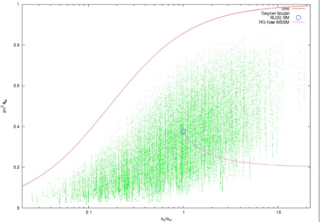
Gauge coupling ratios

These files are needed as input by the program Kac in order to examine each of the 19000 Standard Model spectra. These are just Standard Model brane configurations, not solutions to the tadpole conditions.

This is a zipped archive containing two files. The models.list file can only be read by version 8.08065 or higher of Kac. The models.stat file is partly obsolete. It contains statistics about 19345 of the 32810 models only. Messages about this file may be ignored.

1. Models.list
   

2. Models.stat
   

The file Models.list contains full details of each of the 19345 chiral spectrum types that we found. It is not really human-readable. To see concrete examples, run the program Kac and type the command “browse standard_model x”, where x the spectrum of interest. This command re-builds the entire spectrum from stored boundary labels, for just one particular example (usually the first one for which a certain  spectum type was found). The command “browse adks x” can be used to just display the chiral spectrum type, without an explicit realization.

The program will look in a user-definable directory for the three “Models” files listed above. This directory can be set with the command “set modeldir”.

The Gepner models are identified by a concatenation of the levels, for example (1,1,1,1,7,16) becomes 1111716. If the levels are in ascending order, this assignment is unique (although occasionally confusing).

MIPF numbers, orientifold numbers and boundary numbers have no intrinsic meaning, but are known to the program Kac. Note that these numbers have changed in different versions of Kac. Please use version 8 to get correct answers. If boundary d has the value -1 this means that the standard model is made with only three boundary states.

Note that the spectrum numbers can go to 20079, but only for 19345 of these numbers there are valid spectra (some invalid spectra where inadvertently accepted and assigned a number in an early stage).

The Models.stat file has all valid spectra ordered by total occurrence frequency. The entries in this file are respectively

1. Sequential number
   

2. Spectrum number (as above)
   

3. Total frequency (number of boundary state combinations in the data base)
   

4. MIPF frequency (number of distinct MIPFs containing this spectrum)
   

5. Spectrum type indicator
   

6. Tadpole solution indicator
   
   

The “spectrum type indicator” gives information on the Chan-Paton groups and the representations. For example, U3U2S2U1_AAVS means that the CP group is
U(3) × U(2) × Sp(2) × U(1), that there are chiral anti-symmetric tensors in the first two factors, chiral symmetric ones in the last one, whereas in the third factor all chiral matter is in the vector (or singlet) representation (“T” indicates that both symmetric and anti-symmetric tensors are present).

The tadpole solution indicator is

-----   if no solution was found for a given spectrum
*****   if a solution was found, and
#####   if a solution was found without extra “hidden” branes.

The actual tadpole solution files are not electronically available, since the MIPF, orientifold and boundary labels may have changed after they were computed.

They are available on request.

Results based on the paper

Orientifolds, hypercharge embeddings and the Standard Model

(with Anastasopoulos, Dijkstra and Kiritsis, 2006)

Orientifold Spectra:

Madrid Models

Orientifold Spectra:

General 3 and 4-stack models

Heterotic Spectra:

Gepner models with broken SO(10)

This database unpacks into a set of 325 directories, each of which corresponds to a certain combination of N=2 minimal models, fermionic building blocks or

permutation orbifold building blocks.

Each of these directories contains some sub-directories, which contain spectra for either the standard tensor product, exceptional MIPFs or lifted CFTs.

The naming convention for the directories is determined by the choice of  of the right-moving (fermionic sector) CFT.

Tensor combinations. A tensor product combination is denoted {C1_C2_C3 .... CN},

where C1,... denote a CFT building block. Minimal model building

blocks are denoted by a single number, and are not separated by underscores.
All other building blocks are separated by underscores.

Building Blocks:

PN denotes the permutation orbifold of the k=N minimal models.

FN denotes a fermionic building block.

FF_Modelpq denotes a full fermionic c=9 combination.

The first two are defined in the file SusyPerm.proc and the second in Fermi.proc

in the procedures directory. These procedures can be read by Kac using the load
command. The FF_Model definitions are yet not available on-line.

Directory names: The main directory for a given right-moving CFT is denoted

A_Tensor{C1_C2_C3 .... CN}

The character “A” is used to distinguish different runs, but plays no role here.

Sub-directory names: The subdirectories of A_Tensor{C1_C2_C3 .... CN}
are named according to the subcases considered: various lifts of the left-moving
sector and/or exceptional invariants. A typical name is

{C1_C2_C3 .... CN}AAAEA^7

This means that an exceptional invariant is used in the fourth factor,
and a diagonal invariant in factors 1,2,3 and 5. The only exceptional
invariants that can occur are the ones of the minimal models at levels
10, 16 and 28. The symbol “^7” means that the seventh factor of the
complete tensor product is lifted. The complete tensor product is

            A2 ⊗ A1 ⊗ U30 ⊗ U20 ⊗ C1 ⊗ .... ⊗ CN
Hence the seventh factor is the third one of the internal sector.

“^4” means lifting of U20 (B-L lifting). Second and third lifts of the
same factor are denoted “~4” or “_4” respectively.

Files: These sub-directories contain the following files

1. .spec_sum    contains the spectrum data
   

2. .origin      contains simple current combinations needed to
                reproduce certain spectra
   

3. .project     contains strings identifying the project
   

The content of the spec_sum file is as follows

Column 1   Number of families

Column 2   Number of Q mirror pairs  

Column 3   Number of U mirror pairs  

Column 4   Number of D mirror pairs  

Column 5   Number of L mirror pairs  

Column 6   Number of E mirror pairs

Column 7   Number of Standard model singlets

Column 8   Number of vector bosons

Column 9   Algebra type (see below)

Column 10  Electric charge quantization (see below)  

Column 11  B-L anomaly (0 = NO, 1 = YES)

Column 12  Origin of spectrum (-1: spectrum was not found).

Column 13  Origin of mirror spectrum (-1: not found).

Column 14  Total number of occurrences of the spectrum plus

           its mirror

Example: the A-invariant of the {3888} Gepner model gives rise to a

spectrum with Hodge number h21=145 and h11=1.  The mirror spectrum has these
numbers inverted. In file {3888}AAAA.spec_sum we see that this spectrum was
found for simple current combination 24, whereas the mirror was found for combination 6324. Both can be found in the .origin file. Higher numbers usually

imply that these spectra were found later and are less common. Although mirror symmetry is guaranteed to be an exact symmetry of the list of spectra, because the scans were not exhaustive it may happen that some mirrors were not found (yet).

These are indicated by a -1 in columns 12 or 13.

Algebra type: This is a number ranging from 0 to 7 defined in the paper

Standard Gepner models. Nr. 7 is SO(10), 6 is Pati-Salam and 4

is SU(5).

Charge quantization: This specifies which fractional charges occur in the massless

spectrum. The possibilities are

1. •0   Only integral charge
   

2. •1   Multiples of 1/6
   

3. •2   Multiples of 1/3
   

4. •3   Multiples of 1/2
   

If this number is different from the expectation based on the CFT, the numbers are
enlarged by 10 for extra emphasis. In particular, “10” implies anomalous absence

of massless fractionally charged particles in a CFT that does allow them.

Counting: All numbers in columns 1...8 are obtained by adding up all the
dimensions of the representations in the “hidden” sector, by which we mean all

factors in the gauge group other than SU(3) × SU(2) × U(1).

Exotic Spectra: If the number of families is listed as -1, then the spectrum

contains chiral, fractionally charged particles. All these spectra are lumped

together, and in the last column their total occurrence frequency is listed.

Non-chiral spectra: If the number of families is listed as 0, there are no chiral

exotics and no families. Then the spectrum is completely non-chiral w.r.t.
SU(3) × SU(2) × U(1). All these spectra are lumped together as in the foregoing
case.

Origin: This file contains lines of the form

Nr. current1 current2 current 3 ... | matrix elements of X

where Nr. is the number found in columns 12 or 13 of the .spec_sum file, and the
currents are a list of N numbers that are simple currents in the N factors in the
tensor product. If there are M currents, the M2 matrix elements of X are given.

The lines in this file can be read in by Kac to recompute the spectrum.

Project: This file contains the aforementioned project names, as well as a TeX
string that can be used in TeX output, and the original name of the project directory

at the time the computations were done.

Example file: This example file can be used as Kac input. It will regenerate the spectrum of interest.

Database

Model Data Base